Chapter 2 Probability of success model

Our first model can be used to address problems such as:

• RQ1-a: What is the probability of each algorithm solving a problem at precision \(\epsilon \leq 0.1\)?
• RQ1-b: What is the impact of noise in the probability of success of each algorithm at precision \(\epsilon \leq 0.1\)?

2.1 RQ1 Data preparation

We start importing the dataset

dataset <- readr::read_csv('./data/statscomp.csv')

Let’s select only the columns that interests us. Note we use "" to select some of the columns because they have “-” in the column name

dataset<-dplyr::select(dataset, Algorithm, CostFunction, SD, MaxFevalPerDimensions, simNumber, SolveAt1, "SolveAt1e-1","SolveAt1e-3","SolveAt1e-6", OptimizationSuccessful)

Let’s do some basic transformation

1 - We select only the cases where the optimization completed 2 - We convert True to 1 and 0 to false 3 - We group by the algorithms, functions, SD, and budget so we can summarize and create aggregated data 4 - We create an index of each algorithm and the cost functions. This is basically creating a map of NelderMead=1, PSO=2 etc… This makes things easier to work in Stan. For that we use the function create_index from the utils.R file
5 - We drop the columns we wont use 6 - Get an array with the names of the benchmark functions and the algorithms (to create nicer plots later with lengend)

Since we are only looking at 1e-1 for the precision we comment the other lines

d <- dataset %>% 
  dplyr::filter(OptimizationSuccessful==TRUE) %>%
  dplyr::mutate(
      solvedAt1e1=as.integer(dataset$"SolveAt1e-1"),
      budget=MaxFevalPerDimensions)  %>% 
  dplyr::group_by(Algorithm, CostFunction, SD, budget) %>% 
    dplyr::summarize(
      solvedAt1e1=sum(solvedAt1e1),
      N=n()) %>% 
  dplyr::ungroup() %>%
  dplyr::mutate(AlgorithmID=create_index(Algorithm),
                CostFunctionID=create_index(CostFunction)) %>% 
    dplyr::select(Algorithm,AlgorithmID, CostFunction, CostFunctionID, SD, budget, N,
                  y=solvedAt1e1,
                  )

#List of algorithms
bm <- get_index_names_as_array(d$CostFunction)
algorithms <- get_index_names_as_array(d$Algorithm)

Lets preview a sample of the data set

kable(dplyr::sample_n(d,size=10),"html", booktabs=T, format.args = list(scientific = FALSE), digits = 3) %>% 
  kable_styling(bootstrap_options = c("striped", "hover", "condensed")) %>% 
  kableExtra::scroll_box(width = "100%")

Algorithm	AlgorithmID	CostFunction	CostFunctionID	SD	budget	N	y
RandomSearch2	7	ChenV	3	3	20	10	0
PSO	5	WhitleyN6	28	0	20	10	0
SimulatedAnnealing	8	Schwefel2d26N6	19	3	100000	10	0
NelderMead	4	LunacekBiRastriginN6	9	3	1000	10	0
PSO	5	StrechedVSineWave2N	23	3	10000	10	0
PSO	5	Schwefel2d21N6	17	3	100	10	0
CuckooSearch	2	ZakharovN2	30	3	1000	10	0
DifferentialEvolution	3	StrechedVSineWave2N	23	0	10000	10	10
DifferentialEvolution	3	Schwefel2d21N6	17	0	100000	10	10
CMAES	1	Giunta	8	3	1000	10	1

2.2 RQ1 Stan model

The Stan model is specified in the file: './stanmodels/probsuccess.stan'. Note that at the end of the model we commented the generated quantities. This block generates the predictive posterior y_rep and the log likelihood, log_lik. These values are useful in diagnosing and validating the model but the end file is extremely large (~1Gb for 2000 iterations) and make many of the following calculations slow. If the reader wants to see these values is just to uncomment and run the stan model again

print_stan_code('./stanmodels/probsuccess.stan')

// Probability of success model
// Author: David Issa Mattos
// Date: 16 June 2020
//
//

data {
 int <lower=1> N_total; // Sample size
 int y[N_total]; // Result of the binomial
 int N_draw[N_total]; // Number of draws in the binomial
 
 real x_noise[N_total];//predictor for noise
 
 //To model each algorithm independently
 int <lower=1> N_algorithm; // Number of algorithms
 int algorithm_id[N_total]; //vector that has the id of each algorithm
 
 //To model the influence of each benchmark
 int <lower=1> N_bm;
 int bm_id[N_total];
}

parameters {
  //Fixed effect
  real a_alg[N_algorithm];//the mean effect given by the algorithms
  real b_noise[N_algorithm];//slope for the noise

  // //Random effect. The effect of the benchmarks
  real a_bm_norm[N_bm];//the mean effect given by the base class type
  real<lower=0> s;//std for the random effects
  
}

model {
  real p[N_total];
  
  //Fixed effect
  a_alg ~ normal(0,5);
  b_noise ~ normal(0,5);

  // //Random effects
  s ~ exponential(0.1);
  a_bm_norm ~ normal(0,1);

  for (i in 1:N_total)
  {
    
     p[i] = a_alg[algorithm_id[i]]+ a_bm_norm[bm_id[i]]*s + b_noise[algorithm_id[i]] * x_noise[i];
  }
  
  //Equivalent to: y~binomial(N, inverse_logit(a+bx=alpha))
  y ~ binomial_logit(N_draw,p);
}

//Uncoment this part to get the posterior predictives and the log likelihood
//But note that it takes a lot of space in the final model
// generated quantities{
//   vector [N_total] y_rep;
//   vector[N_total] log_lik;
//   
//   for(i in 1:N_total){
//     real p;
//     p = a_alg[algorithm_id[i]]+ a_bm_norm[bm_id[i]]*s + b_noise[algorithm_id[i]] * x_noise[i];
// 
//     y_rep[i] = binomial_rng(N_draw[i], inv_logit(p));
//     
//     //Log likelihood
//      log_lik[i] = binomial_lpmf(y[i] | N_draw[i], inv_logit(p));
//   }
// }

Let’s compile and start sampling with the Stan function. In the data folder you can find the specific data used to fit the model after all transformations "./data/probsuccsess-data.RDS"

standata <- list(
  N_total = nrow(d),
  y = d$y,
  N_draw = d$N,
  x_noise = d$SD,
  N_algorithm = length(algorithms),
  algorithm_id =d$AlgorithmID,
  N_bm = length(bm),
  bm_id = d$CostFunctionID)
saveRDS(standata, file = "./data/probsuccsess-data.RDS")

For computation time sake we are not running this chunk every time we compile this document. From now on we will load from the saved Stan fit object in the data folder. However, when we change our model or the data we can just run this chunk separately.

standata<-readRDS("./data/probsuccsess-data.RDS")
probsuccess.fit <- stan(file = './stanmodels/probsuccess.stan',
                     data=standata,
                     chains = 4,
                     warmup = 200,
                     iter = 3000)
saveRDS(probsuccess.fit, file = "./data/probsuccsess-fit.RDS")

2.3 RQ1 Diagnosis

2.3.1 RQ1 Chains convergence

The first step is to evaluate the convergence of the chains. We will look now only for the slopes, algorithms intercept and the standard deviation of the random effects (and not each intercept of the random effects)

a_alg <- c("a_alg[1]",
           "a_alg[2]",
           "a_alg[3]",
           "a_alg[4]",
           "a_alg[5]",
           "a_alg[6]",
           "a_alg[7]",
           "a_alg[8]")
b_noise <- c("b_noise[1]",
             "b_noise[2]",
             "b_noise[3]",
             "b_noise[4]",
             "b_noise[5]",
             "b_noise[6]",
             "b_noise[7]",
             "b_noise[8]")
rstan::traceplot(probsuccess.fit, pars=a_alg)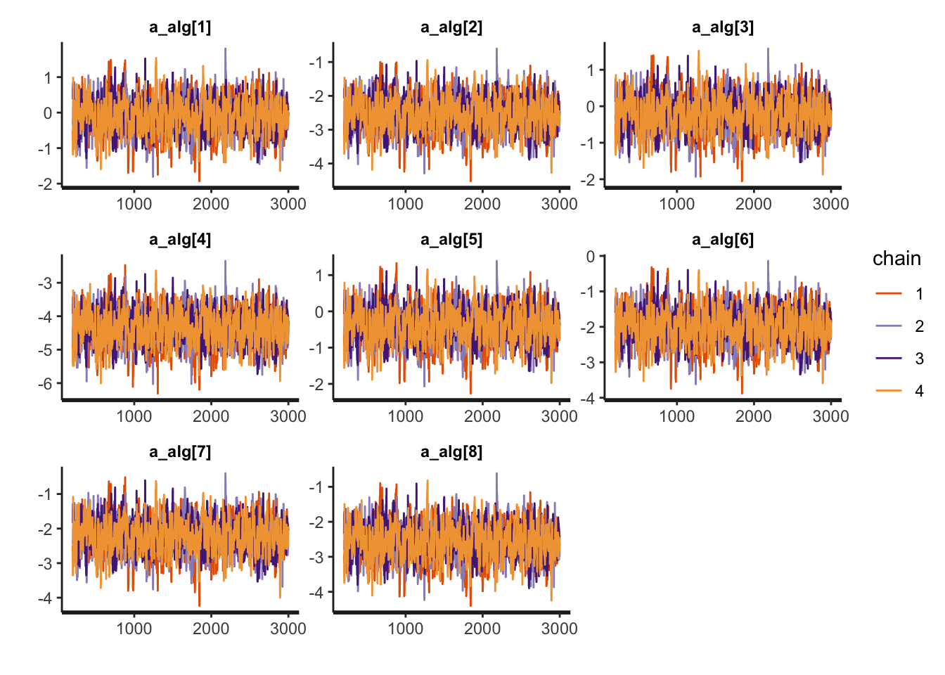

rstan::traceplot(probsuccess.fit, pars=b_noise)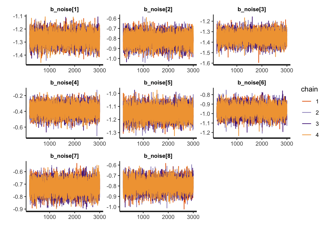

rstan::traceplot(probsuccess.fit, pars=c('s'))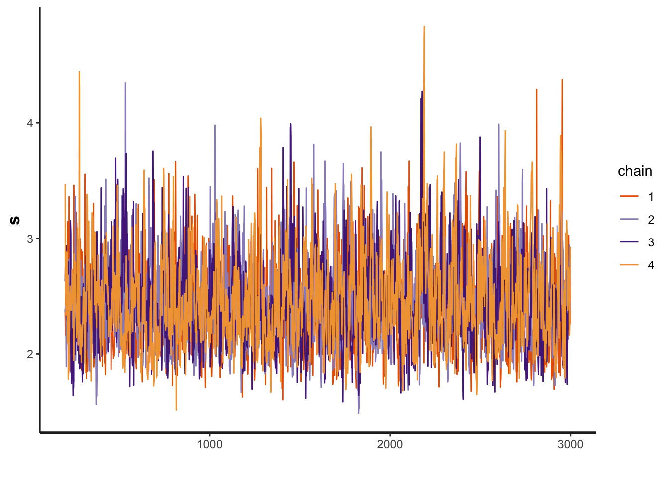

Another diagnosis is to look at the Rhat. If Rhat is greater than 1.05 it indicates a divergence in the chains (they did not mix well). The table below shows a summary of the sampling.

kable(summary(probsuccess.fit)$summary) %>% 
  kable_styling(bootstrap_options = c('striped',"hover", "condensed" )) %>% 
  kableExtra::scroll_box(width = "100%")

	mean	se_mean	sd	2.5%	25%	50%	75%	97.5%	n_eff	Rhat
a_alg[1]	-0.1016770	0.0141859	0.4511590	-0.9986581	-0.3944800	-0.1079857	0.1956272	0.7748758	1011.456	1.0007354
a_alg[2]	-2.5516066	0.0142459	0.4563417	-3.4560617	-2.8523292	-2.5527132	-2.2471997	-1.6730424	1026.124	1.0009415
a_alg[3]	-0.2139745	0.0142481	0.4513760	-1.1136926	-0.5092907	-0.2159365	0.0889257	0.6489137	1003.611	1.0007939
a_alg[4]	-4.3498335	0.0142878	0.4667423	-5.2926288	-4.6576410	-4.3486295	-4.0362012	-3.4514857	1067.149	1.0007534
a_alg[5]	-0.3943603	0.0142332	0.4506022	-1.2874160	-0.6869869	-0.3994464	-0.0884889	0.4724644	1002.264	1.0009414
a_alg[6]	-2.0070362	0.0142076	0.4539332	-2.9122092	-2.3013030	-2.0129352	-1.7030975	-1.1352872	1020.806	1.0008781
a_alg[7]	-2.2163631	0.0142042	0.4537016	-3.1183583	-2.5133972	-2.2204326	-1.9159819	-1.3441906	1020.248	1.0009555
a_alg[8]	-2.5625822	0.0142418	0.4562100	-3.4753740	-2.8617582	-2.5668217	-2.2559160	-1.6908949	1026.123	1.0008100
b_noise[1]	-1.2728595	0.0004634	0.0464911	-1.3649835	-1.3042495	-1.2727833	-1.2419386	-1.1808717	10064.607	1.0003304
b_noise[2]	-0.8111614	0.0005341	0.0594260	-0.9269817	-0.8512298	-0.8108461	-0.7706404	-0.6960778	12378.857	0.9998278
b_noise[3]	-1.3531582	0.0004555	0.0498441	-1.4530193	-1.3862144	-1.3528896	-1.3200088	-1.2545062	11973.466	1.0003042
b_noise[4]	-0.3851807	0.0006594	0.0708802	-0.5254143	-0.4334606	-0.3844210	-0.3357693	-0.2486244	11553.895	0.9998575
b_noise[5]	-1.1483855	0.0004288	0.0471090	-1.2413071	-1.1803177	-1.1475632	-1.1166922	-1.0569722	12068.645	0.9999617
b_noise[6]	-0.9653479	0.0005154	0.0567297	-1.0794613	-1.0029451	-0.9644473	-0.9267742	-0.8573317	12113.240	0.9999536
b_noise[7]	-0.7231598	0.0005147	0.0521852	-0.8278536	-0.7579466	-0.7223159	-0.6875584	-0.6217345	10280.685	0.9998671
b_noise[8]	-0.7934309	0.0006002	0.0579600	-0.9074668	-0.8320577	-0.7937229	-0.7548121	-0.6780034	9326.707	1.0000572
a_bm_norm[1]	-0.5515980	0.0059809	0.2113896	-0.9712815	-0.6922152	-0.5481803	-0.4065674	-0.1432695	1249.219	1.0005773
a_bm_norm[2]	-1.3857790	0.0072688	0.3110012	-2.0315335	-1.5876596	-1.3696647	-1.1724448	-0.8177882	1830.642	1.0004815
a_bm_norm[3]	-0.6135924	0.0059932	0.2138498	-1.0370821	-0.7578332	-0.6099309	-0.4669450	-0.1978411	1273.226	1.0007982
a_bm_norm[4]	0.6996375	0.0065183	0.2143535	0.2882285	0.5533039	0.6956576	0.8438217	1.1273589	1081.413	1.0011373
a_bm_norm[5]	-0.9190532	0.0063871	0.2451850	-1.4221268	-1.0826093	-0.9142283	-0.7500079	-0.4543208	1473.602	1.0004336
a_bm_norm[6]	-0.1266989	0.0057661	0.1905645	-0.5002489	-0.2576990	-0.1251113	0.0010672	0.2486333	1092.226	1.0005111
a_bm_norm[7]	2.0929329	0.0098459	0.3562187	1.4022113	1.8483216	2.0869635	2.3308668	2.8104401	1308.946	1.0019514
a_bm_norm[8]	1.4163381	0.0079819	0.2778883	0.8720145	1.2260972	1.4104389	1.6037712	1.9676857	1212.061	1.0016224
a_bm_norm[9]	-2.2875170	0.0080868	0.5070058	-3.3784938	-2.6042096	-2.2496205	-1.9305845	-1.4020841	3930.757	1.0003584
a_bm_norm[10]	0.0376740	0.0057984	0.1890303	-0.3267560	-0.0909227	0.0381280	0.1632858	0.4111242	1062.770	1.0008355
a_bm_norm[11]	-0.4683589	0.0058892	0.2054966	-0.8814239	-0.6047223	-0.4628744	-0.3299558	-0.0697175	1217.572	1.0004397
a_bm_norm[12]	0.9705429	0.0072309	0.2352270	0.5211149	0.8117004	0.9658386	1.1296289	1.4391891	1058.256	1.0014069
a_bm_norm[13]	0.1111258	0.0058348	0.1895685	-0.2518913	-0.0206515	0.1106819	0.2360902	0.4897085	1055.563	1.0006293
a_bm_norm[14]	-0.4185043	0.0058612	0.2020018	-0.8150537	-0.5543865	-0.4170919	-0.2820809	-0.0200522	1187.764	1.0004502
a_bm_norm[15]	-0.2120039	0.0057779	0.1931704	-0.5875451	-0.3435861	-0.2108279	-0.0835340	0.1704687	1117.724	1.0004975
a_bm_norm[16]	0.0582553	0.0057948	0.1899707	-0.3051919	-0.0713240	0.0577533	0.1855058	0.4365644	1074.708	1.0007318
a_bm_norm[17]	-0.0945615	0.0058098	0.1905650	-0.4616333	-0.2244295	-0.0938981	0.0338356	0.2816415	1075.888	1.0006509
a_bm_norm[18]	0.3553886	0.0060492	0.1962915	-0.0150112	0.2217934	0.3541406	0.4875904	0.7474879	1052.943	1.0007216
a_bm_norm[19]	-1.3873544	0.0071574	0.3144653	-2.0341171	-1.5904221	-1.3696656	-1.1671590	-0.8205984	1930.342	1.0006691
a_bm_norm[20]	-0.2103035	0.0057874	0.1925856	-0.5825628	-0.3399080	-0.2079499	-0.0814456	0.1685257	1107.335	1.0007190
a_bm_norm[21]	0.0374586	0.0057911	0.1888960	-0.3244013	-0.0918735	0.0378206	0.1633785	0.4096106	1063.953	1.0007178
a_bm_norm[22]	0.4262087	0.0061486	0.1989057	0.0477541	0.2899258	0.4231280	0.5578995	0.8254036	1046.516	1.0011291
a_bm_norm[23]	-0.2208615	0.0057839	0.1927261	-0.5929206	-0.3516246	-0.2213745	-0.0911591	0.1589538	1110.306	1.0006586
a_bm_norm[24]	0.9181966	0.0069786	0.2314096	0.4725721	0.7597149	0.9153235	1.0732483	1.3825348	1099.586	1.0014348
a_bm_norm[25]	-0.4800747	0.0058778	0.2060577	-0.8903264	-0.6193752	-0.4793265	-0.3426119	-0.0764864	1228.989	1.0007175
a_bm_norm[26]	1.8127547	0.0090502	0.3223532	1.1907146	1.5925470	1.8072705	2.0297038	2.4651831	1268.663	1.0017888
a_bm_norm[27]	-0.3950165	0.0058627	0.2010451	-0.7896719	-0.5304012	-0.3915179	-0.2564086	-0.0006536	1175.971	1.0004427
a_bm_norm[28]	-1.5823227	0.0078727	0.3510577	-2.3267529	-1.8102101	-1.5614566	-1.3363711	-0.9473444	1988.408	1.0008761
a_bm_norm[29]	0.4734666	0.0062045	0.2008774	0.0930725	0.3343172	0.4734256	0.6092113	0.8729607	1048.224	1.0011553
a_bm_norm[30]	0.7791124	0.0067026	0.2195527	0.3600034	0.6284312	0.7741367	0.9296758	1.2156303	1072.990	1.0013464
s	2.4396697	0.0091963	0.3666749	1.8524855	2.1797734	2.3975453	2.6487166	3.2807386	1589.761	1.0026073
lp__	-5600.1110570	0.1389985	6.2045095	-5613.2707018	-5604.0278224	-5599.7723066	-5595.7819986	-5588.9259626	1992.483	1.0021429

2.4 RQ1 Results and Plots

First lets get the HPDI of every parameter. We do this with the helper function from utils.R. But the function is quite simple. It just converts the stanmodel object to an object that the coda package can read (and do some renaming). Alternatively we can use the HDInterval package.

Then we restrict to the algorithms, them to the slopes, then to the other parameters. We create different data frames that we use to plot with ggplot pointrange

hpdi <- get_HPDI_from_stanfit(probsuccess.fit)
hpdi_oddsratio <- hpdi
hpdi_oddsratio$Mean <- exp(hpdi$Mean)
hpdi_oddsratio$HPDI.lower <- exp(hpdi$HPDI.lower)
hpdi_oddsratio$HPDI.higher <- exp(hpdi$HPDI.higher)


hpdi_oddsratio_algorithm <- hpdi_oddsratio %>% 
      dplyr::filter(str_detect(Parameter, "a_alg\\[")) %>%
      dplyr::mutate(Parameter=algorithms) #Changing to the algorithms labels

hpdi_oddsratio_b_noise <- hpdi_oddsratio %>% 
      dplyr::filter(str_detect(Parameter, "b_noise\\[")) %>%
      dplyr::mutate(Parameter=algorithms) #Changing to the algorithms labels

hpdi_s <- hpdi %>% 
      dplyr::filter(Parameter=='s') 


p_alg<-ggplot(data=hpdi_oddsratio_algorithm, aes(x=Parameter))+
  geom_pointrange(aes(
    ymin=HPDI.lower, 
    ymax=HPDI.higher, 
    y=Mean))+
  labs(y="Odds ratio for intercept", x="Algorithm")+
  coord_flip()
p_alg + plot_annotation(title = 'HPDI interval for the algorithms OR')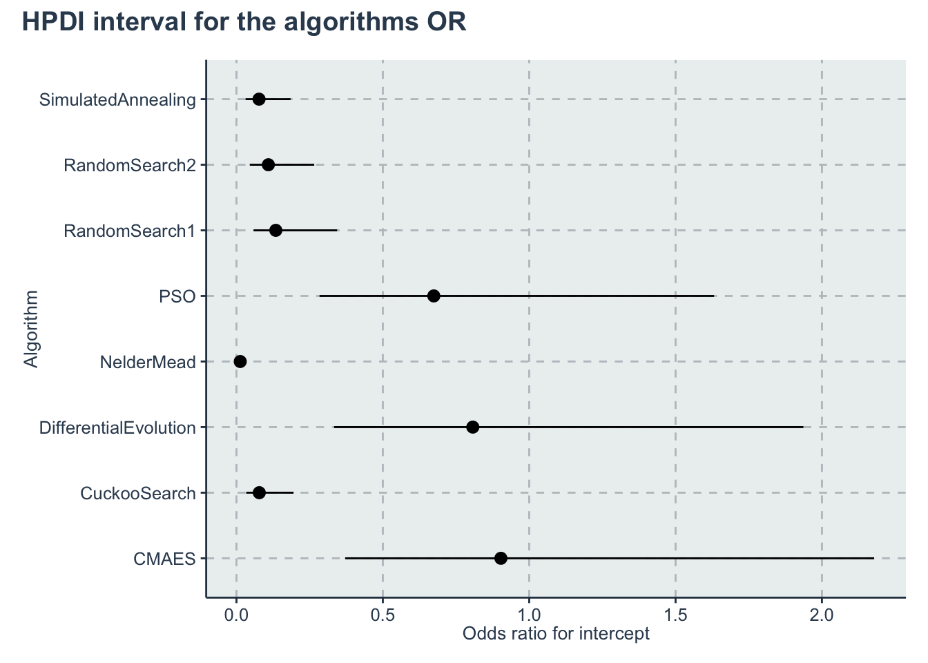

p_noise <- ggplot(data=hpdi_oddsratio_b_noise, aes(x=Parameter))+
  geom_pointrange(aes(
    ymin=HPDI.lower, 
    ymax=HPDI.higher, 
    y=Mean))+
  labs( y="Odds ratio for b_noise", x="Parameter")+
  coord_flip()+
  theme()
p_noise + plot_annotation(title = 'HPDI interval for the noise coefficients OR')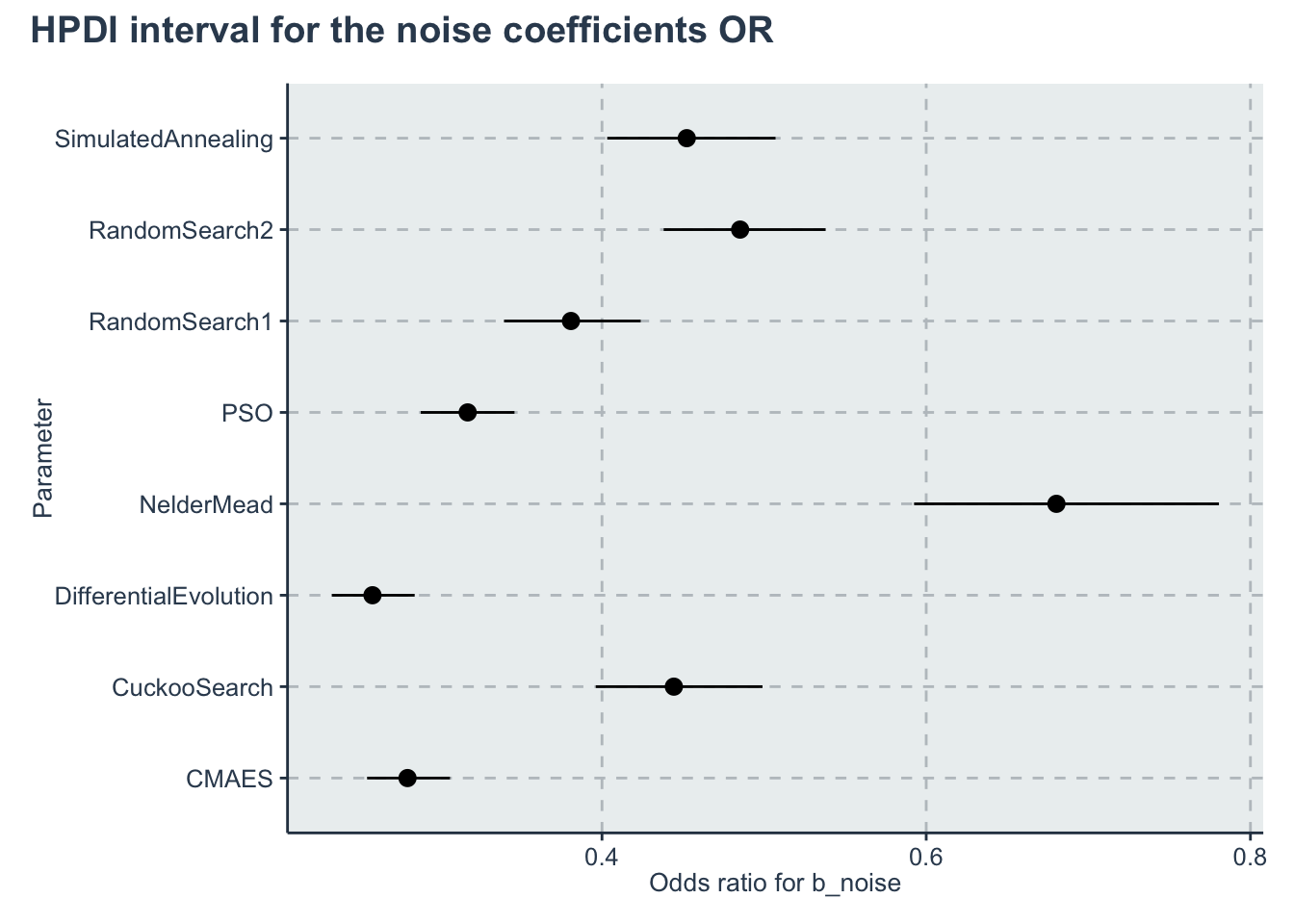

p_s <- ggplot(data=hpdi_s, aes(x=Parameter))+
  geom_pointrange(aes(
    ymin=HPDI.lower, 
    ymax=HPDI.higher, 
    y=Mean))+
  labs(y="s", x="Parameter")+
  coord_flip()
p_s + plot_annotation(title = 'HPDI interval for s')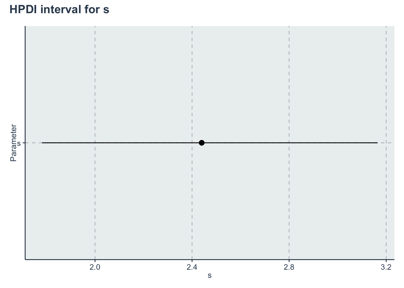

Creating an output table

algreduced <- c("CMAES", "Cuckoo", "DiffEvol.", "NelderM.", "PSO", "RandomS1","RandomS2", "SimAnneal")
rename_pars <- c(
  paste(rep('a_',length(algorithms)),algreduced, sep = ""),
  paste(rep('b_',length(algorithms)),algreduced, sep = ""),
  's')

t<-create_table_model(probsuccess.fit, pars = c(a_alg, b_noise, 's'), renamepars =  rename_pars)

t<- t %>% 
  mutate('OR Mean' = exp(Mean),
         'OR HPD low' = exp(HPDI.lower),
         'OR HPD high' = exp(HPDI.higher))
colnames(t)<-c("Parameter", "Mean", "HPD low", "HPD high",'OR Mean','OR HPD low','OR HPD high')

saveRDS(t,'./statscomp-paper/tables/datafortables/probsuccess-par-table.RDS')