Chapter 5 Function Evaluation to converge

In this section, we will consider the Cox’s Proportional Hazard model for analyzing the time to converge to a a solution (in number of iterations).

RQ4-a: What is the average number of function evaluations taken by an algorithm to converge to a solution at a precision of \(\epsilon=0.1\), with a budget of 100,000 function evaluations per dimension?
RQ4-b: What is the impact of noise in the number of function evaluations taken by an algorithm to converge to a solution at a precision of \(\epsilon=0.1\), with a budget of 100,000 function evaluations per dimension?

5.1 RQ4 Data preparation

We start importing the dataset

dataset <- readr::read_csv('./data/statscomp.csv')

Filtering the data that we want and applying some transformations. The Event variable will indicate if it was censored or not.

d <- dataset %>% 
  dplyr::filter(OptimizationSuccessful==TRUE & MaxFevalPerDimensions==100000 & (Algorithm=="PSO"|Algorithm=="CMAES"|Algorithm=="DifferentialEvolution"|Algorithm=="RandomSearch1")) %>% 
  dplyr::select(Algorithm, CostFunction, Event="SolveAt1e-1", simNumber, Ndimensions, SD, SolvedAtIteration="SolveEarlierAt1e-1") %>% 
  dplyr::mutate(y=SolvedAtIteration/Ndimensions,
                Event=as.integer(Event),
                CostFunctionID=create_index(CostFunction),
                AlgorithmID=create_index(Algorithm)) %>% 
  dplyr::select(Algorithm, AlgorithmID, CostFunction, CostFunctionID, SD, Event, y,-simNumber,-SolvedAtIteration, -Ndimensions)

algorithms<-get_index_names_as_array(d$Algorithm)
bm <- get_index_names_as_array(d$CostFunction)

The data should look like this:

kable(dplyr::sample_n(d,size=10),"html", booktabs=T, format.args = list(scientific = FALSE), digits = 3) %>% 
  kable_styling(bootstrap_options = c("striped", "hover", "condensed")) %>% 
  kableExtra::scroll_box(width = "100%")

Algorithm	AlgorithmID	CostFunction	CostFunctionID	SD	Event	y
PSO	3	DiscusN2	6	0	1	44850.000
RandomSearch1	4	Schwefel2d26N6	19	0	0	NA
DifferentialEvolution	2	ExponentialN2	7	3	0	0.500
CMAES	1	DiscusN2	6	0	0	NA
RandomSearch1	4	Tripod	27	3	0	NA
CMAES	1	SphereN6	22	0	1	40.333
PSO	3	WhitleyN6	28	3	0	NA
CMAES	1	PinterN6	11	3	0	NA
CMAES	1	SphereN6	22	3	0	46.667
PSO	3	Schwefel2d23N6	18	3	0	237.833

5.2 RQ4 Stan model

The Stan model is specified in the file: './stanmodels/timetoconverge.stan'. Note that at the end of the model we commented the generated quantities. This block generates the predictive posterior y_rep and the log likelihood, log_lik. These values are useful in diagnosing and validating the model but the end file is extremely large (~1Gb for 2000 iterations) and make many of the following calculations slow. If the reader wants to see these values is just to uncomment and run the stan model again. Note also the the predictive posterior calculates for censored and non censored data. We can in r restrict and compare the predictive only to the non censored data or even censor it if the prediction is above the budget.

print_stan_code('./stanmodels/timetoconverge.stan')

// Time to converge, Cox regression model
// Author: David Issa Mattos
// Date: 23 June 2020
//
//

data {
 int <lower=1> N_total; // Sample size
 real y[N_total]; // iteration where it was solved
 int event[N_total]; // Indicates if the event occured or not

 //To model each algorithm independently
 int <lower=1> N_algorithm; // Number of algorithms
 int algorithm_id[N_total]; //vector that has the id of each algorithm
 
 //To model the influence of the noise
 real x_noise[N_total];
 
 //To model the influence of each benchmark
 int <lower=1> N_bm;
 int bm_id[N_total];
}

parameters {
  
  //Fixed effect
  real a_alg[N_algorithm];//the mean effect given by the algorithms
  real b_noise[N_algorithm];//effect of noise
  // //Random effect. The effect of the benchmarks
  real a_bm_norm[N_bm];//the mean effect given by the base class type
  real<lower=0> s;//std for the random effects
  
}

model {
  
  
  //Fixed effect
  a_alg ~ normal(0,10);
  
  // //Random effects
  s ~ exponential(0.1);
  a_bm_norm ~ normal(0,1);
  b_noise ~ normal(0,2);

  for (i in 1:N_total)
  {
    //uncensored data
    if(event[i]==1) target += exponential_lpdf(y[i] | exp(a_alg[algorithm_id[i]] + s*a_bm_norm[bm_id[i]] + b_noise[algorithm_id[i]]*x_noise[i])); 
    //censored data
    if(event[i]==0) target += exponential_lccdf(y[i] | exp(a_alg[algorithm_id[i]] + s*a_bm_norm[bm_id[i]] + b_noise[algorithm_id[i]]*x_noise[i]));  
  }
  
}


//Uncoment this part to get the posterior predictives and the log likelihood
//But note that it takes a lot of space in the final model
// //Here we suppose that the predictive data will not be censored.
// //But if it is above the budget we can censor it later
// generated quantities{
//   vector [N_total] y_rep;
//   vector[N_total] log_lik;
//   
//   for(i in 1:N_total){
//     real mu;
//     mu = a_alg[algorithm_id[i]] + s*a_bm_norm[bm_id[i]] + b_noise[algorithm_id[i]]*x_noise[i];
//     y_rep[i]= exponential_rng(mu);
//     
//     //uncensored data
//     if(event[i]==1) log_lik[i]= exponential_lpdf(y[i] | exp(a_alg[algorithm_id[i]] + s*a_bm_norm[bm_id[i]] + b_noise[algorithm_id[i]]*x_noise[i])); 
//     //censored data
//     if(event[i]==0) log_lik[i]= exponential_lccdf(y[i] | exp(a_alg[algorithm_id[i]] + s*a_bm_norm[bm_id[i]] + b_noise[algorithm_id[i]]*x_noise[i]));  
//   }
// }

Let’s compile and start sampling with the Stan function. In the data folder you can find the specific data used to fit the model after all transformations "./data/timetoconverge-data.RDS"

Note that stan does not support NA in the data, so we have two options… We either replace NA for a value and add conditionals in the model (note that this value will not be used). Or we separate the data frame in two parts, censored and not not-censored. We will do the first approach replacing the NA by 0.

dstan<-d %>% 
  dplyr::mutate(y=replace_na(y,0))

standata <- list(
  N_total=nrow(dstan),
  y = dstan$y,
  event = dstan$Event,
  x_noise = d$SD,
  N_algorithm = length(algorithms),
  algorithm_id = dstan$AlgorithmID,
  N_bm = length(bm),
  bm_id = d$CostFunctionID
  )
saveRDS(standata, file = "./data/timetoconverge-data.RDS")

For computation time sake we are not running this chunk every time we compile this document. From now on we will load from the saved Stan fit object. However, when we change our model or the data we can just run this chunk separately

standata<-readRDS("./data/timetoconverge-data.RDS")
timetoconverge_fit <- stan(file = './stanmodels/timetoconverge.stan',
                     data=standata,
                     chains = 4,
                     warmup = 200,
                     iter = 3000)
saveRDS(timetoconverge_fit, file = "./data/timetoconverge-fit.RDS")

5.3 RQ4 Diagnosis

a_alg <- c("a_alg[1]",
           "a_alg[2]",
           "a_alg[3]",
           "a_alg[4]")

b_noise <- c("b_noise[1]",
           "b_noise[2]",
           "b_noise[3]",
           "b_noise[4]")
rstan::traceplot(timetoconverge_fit, pars=a_alg)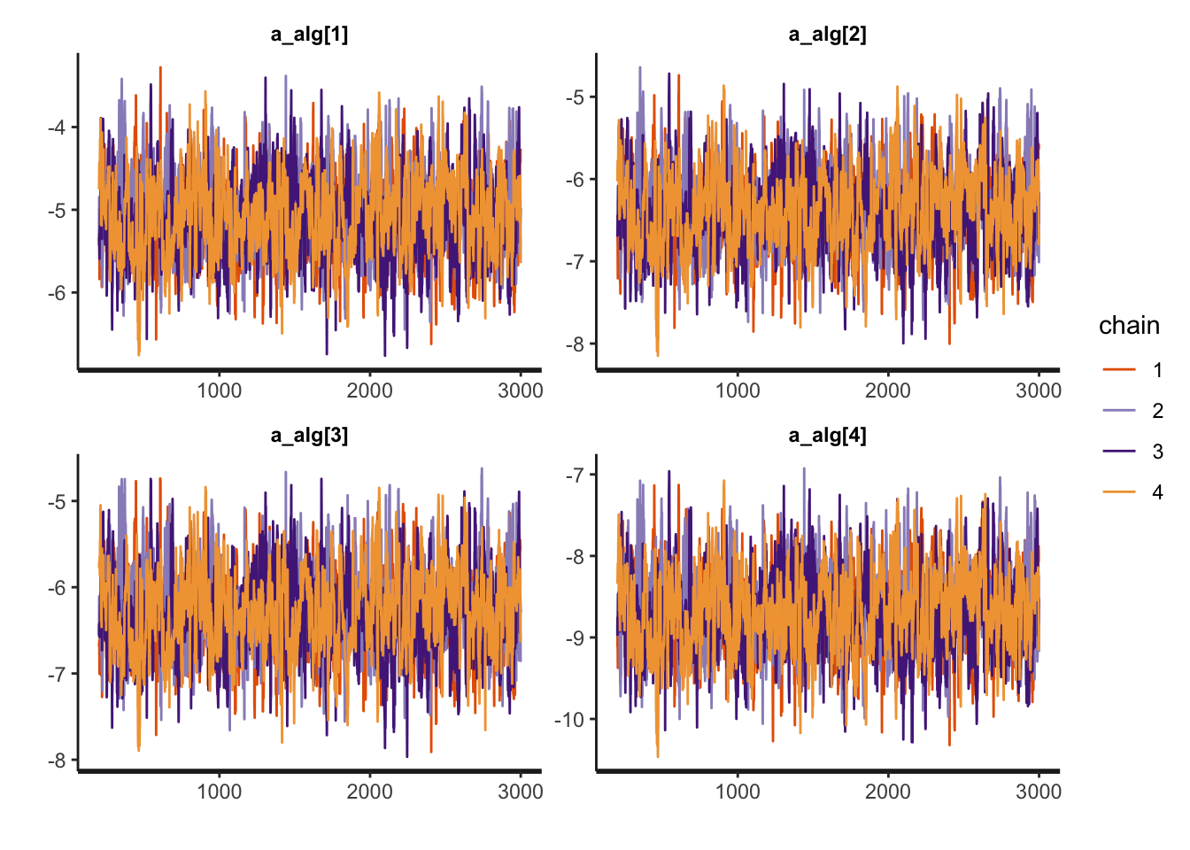

rstan::traceplot(timetoconverge_fit, pars=b_noise)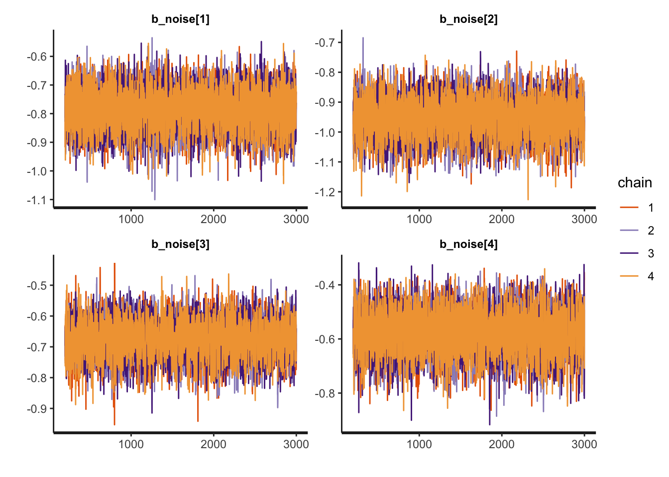

rstan::traceplot(timetoconverge_fit, pars='s')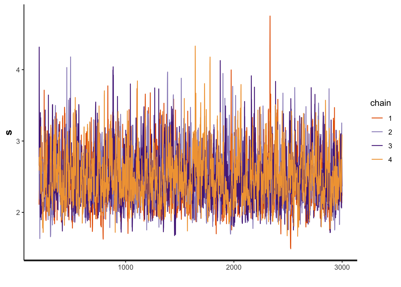

Another diagnosis is to look at the Rhat. If Rhat is greater than 1.05 it indicates a divergence in the chains (they did not mix well). The table below shows a summary of the sampling.

kable(summary(timetoconverge_fit)$summary) %>% 
  kable_styling(bootstrap_options = c('striped',"hover", "condensed" )) %>% 
  kableExtra::scroll_box(width = "100%")

	mean	se_mean	sd	2.5%	25%	50%	75%	97.5%	n_eff	Rhat
a_alg[1]	-5.0748271	0.0148421	0.4735059	-5.9748027	-5.4004954	-5.0811150	-4.7594485	-4.1269815	1017.792	1.0062787
a_alg[2]	-6.3871417	0.0148498	0.4697594	-7.2845576	-6.7112468	-6.3891614	-6.0738266	-5.4345811	1000.714	1.0063466
a_alg[3]	-6.2898339	0.0147225	0.4692970	-7.1799064	-6.6112746	-6.2918339	-5.9776548	-5.3393856	1016.088	1.0060641
a_alg[4]	-8.6911983	0.0150255	0.4779351	-9.6079250	-9.0188308	-8.6949784	-8.3717172	-7.7361202	1011.760	1.0058845
b_noise[1]	-0.7841948	0.0006829	0.0700337	-0.9254156	-0.8292292	-0.7826036	-0.7362581	-0.6519258	10517.588	1.0003918
b_noise[2]	-0.9531764	0.0006549	0.0648313	-1.0847994	-0.9960676	-0.9522515	-0.9085118	-0.8291181	9801.285	0.9996793
b_noise[3]	-0.6750192	0.0007456	0.0618255	-0.8012824	-0.7157411	-0.6735213	-0.6329539	-0.5578453	6875.241	1.0000335
b_noise[4]	-0.5780610	0.0008348	0.0804612	-0.7382183	-0.6322695	-0.5761187	-0.5230502	-0.4264751	9289.680	0.9999791
a_bm_norm[1]	-0.6965849	0.0063953	0.2408707	-1.1898297	-0.8556381	-0.6907584	-0.5320683	-0.2328818	1418.538	1.0038465
a_bm_norm[2]	-0.5777261	0.0068955	0.4316043	-1.5625677	-0.8336753	-0.5360934	-0.2752100	0.1556809	3917.799	1.0009448
a_bm_norm[3]	-0.6236323	0.0063588	0.2271429	-1.0817263	-0.7748316	-0.6180451	-0.4685312	-0.1923110	1275.990	1.0041453
a_bm_norm[4]	0.1265026	0.0058734	0.1951705	-0.2565235	-0.0069494	0.1270324	0.2643450	0.4997121	1104.208	1.0059306
a_bm_norm[5]	-0.5759095	0.0060949	0.2554721	-1.0923145	-0.7454205	-0.5713378	-0.3982293	-0.0911667	1756.939	1.0032683
a_bm_norm[6]	-0.9766402	0.0067009	0.2393889	-1.4608203	-1.1301936	-0.9717149	-0.8151335	-0.5193319	1276.273	1.0039329
a_bm_norm[7]	2.7370066	0.0101284	0.4209890	1.9367581	2.4502287	2.7263716	3.0244169	3.5721570	1727.664	1.0031417
a_bm_norm[8]	1.7538444	0.0079298	0.3113164	1.1560189	1.5404985	1.7501828	1.9682233	2.3553327	1541.290	1.0039046
a_bm_norm[9]	-0.0041220	0.0108223	1.0026192	-1.9926051	-0.6755989	-0.0068539	0.6708510	1.9798202	8582.944	0.9998661
a_bm_norm[10]	-0.4315799	0.0061151	0.2038895	-0.8404470	-0.5705033	-0.4306554	-0.2899537	-0.0433997	1111.691	1.0054807
a_bm_norm[11]	-0.5259654	0.0062813	0.2320727	-1.0016897	-0.6782325	-0.5212058	-0.3696708	-0.0885248	1365.057	1.0039398
a_bm_norm[12]	0.9068971	0.0064833	0.2329520	0.4544769	0.7455659	0.9050496	1.0665512	1.3565692	1291.032	1.0053887
a_bm_norm[13]	-0.4359458	0.0061185	0.2078811	-0.8463867	-0.5740035	-0.4343978	-0.2939291	-0.0382113	1154.354	1.0044905
a_bm_norm[14]	-0.5611604	0.0062895	0.2186831	-0.9921228	-0.7077741	-0.5574438	-0.4103387	-0.1426650	1208.918	1.0037847
a_bm_norm[15]	-0.6093862	0.0061928	0.2186447	-1.0563642	-0.7537575	-0.6074251	-0.4588930	-0.1877069	1246.542	1.0037959
a_bm_norm[16]	-0.1300590	0.0059541	0.1982747	-0.5215199	-0.2645092	-0.1280031	0.0080854	0.2464275	1108.926	1.0054374
a_bm_norm[17]	-0.8254504	0.0064065	0.2261639	-1.2866539	-0.9751358	-0.8233464	-0.6698349	-0.3955225	1246.253	1.0034022
a_bm_norm[18]	0.2086358	0.0058512	0.1968964	-0.1784470	0.0744810	0.2075393	0.3447130	0.5823112	1132.377	1.0058857
a_bm_norm[19]	-0.4961383	0.0064632	0.3014570	-1.1212569	-0.6881725	-0.4841014	-0.2885630	0.0617583	2175.463	1.0012575
a_bm_norm[20]	-0.4030878	0.0061632	0.2137075	-0.8352109	-0.5437513	-0.4023146	-0.2533124	-0.0035589	1202.323	1.0046415
a_bm_norm[21]	-0.6078715	0.0062295	0.2106205	-1.0271393	-0.7478032	-0.6053876	-0.4642284	-0.2029004	1143.133	1.0047761
a_bm_norm[22]	0.8147772	0.0063431	0.2273031	0.3741683	0.6582662	0.8148677	0.9724791	1.2506644	1284.123	1.0051303
a_bm_norm[23]	-0.5624268	0.0062140	0.2145921	-0.9935462	-0.7043190	-0.5604617	-0.4166895	-0.1503493	1192.559	1.0041953
a_bm_norm[24]	0.8505912	0.0064559	0.2302010	0.4029159	0.6899970	0.8482067	1.0106928	1.2894445	1271.473	1.0056251
a_bm_norm[25]	-1.0437646	0.0067559	0.2449729	-1.5429579	-1.2032632	-1.0416170	-0.8773582	-0.5722703	1314.833	1.0035678
a_bm_norm[26]	2.1491961	0.0086831	0.3531701	1.4738920	1.9038174	2.1439157	2.3909719	2.8434322	1654.308	1.0033435
a_bm_norm[27]	-0.4074135	0.0061642	0.2200510	-0.8398117	-0.5532337	-0.4047249	-0.2547040	0.0094274	1274.343	1.0043605
a_bm_norm[28]	-0.8421851	0.0068159	0.4135339	-1.7664022	-1.0984919	-0.8014230	-0.5507585	-0.1228178	3681.056	1.0007621
a_bm_norm[29]	0.3769791	0.0060082	0.2086409	-0.0361264	0.2336479	0.3784831	0.5230282	0.7762157	1205.901	1.0061095
a_bm_norm[30]	0.8778486	0.0065097	0.2327422	0.4259823	0.7175528	0.8777734	1.0409110	1.3204945	1278.271	1.0052698
s	2.4787526	0.0078300	0.3477918	1.9115061	2.2297659	2.4443030	2.6820143	3.2530978	1972.951	1.0021061
lp__	-5484.5180011	0.1232301	5.6597193	-5496.8727218	-5488.1030994	-5484.1825342	-5480.4879169	-5474.5067482	2109.386	1.0011965

5.4 RQ4 Results and Plots

5.4.1 RQ4 Parameters and plots

First lets get the HPDI of every parameter.

Then we restrict to the algorithms, them to the slopes, then to the parameter s

hpdi <- get_HPDI_from_stanfit(timetoconverge_fit)

hpdi_algorithm <- hpdi %>% 
      dplyr::filter(str_detect(Parameter, "a_alg\\[")) %>%
      dplyr::mutate(Parameter=algorithms) #Changing to the algorithms labels

hpdi_noise<- hpdi %>% 
      dplyr::filter(str_detect(Parameter, "b_noise\\[")) %>%
      dplyr::mutate(Parameter=algorithms) #Changing to the algorithms labels

hpdi_s <- hpdi %>% 
      dplyr::filter(Parameter=='s')


p_alg<-ggplot(data=hpdi_algorithm, aes(x=Parameter))+
  geom_pointrange(aes(
    ymin=HPDI.lower, 
    ymax=HPDI.higher, 
    y=Mean))+
  labs(y="a_alg", x="Algorithm")+
  coord_flip()
p_alg + plot_annotation(title = 'HPDI interval for the algorithms')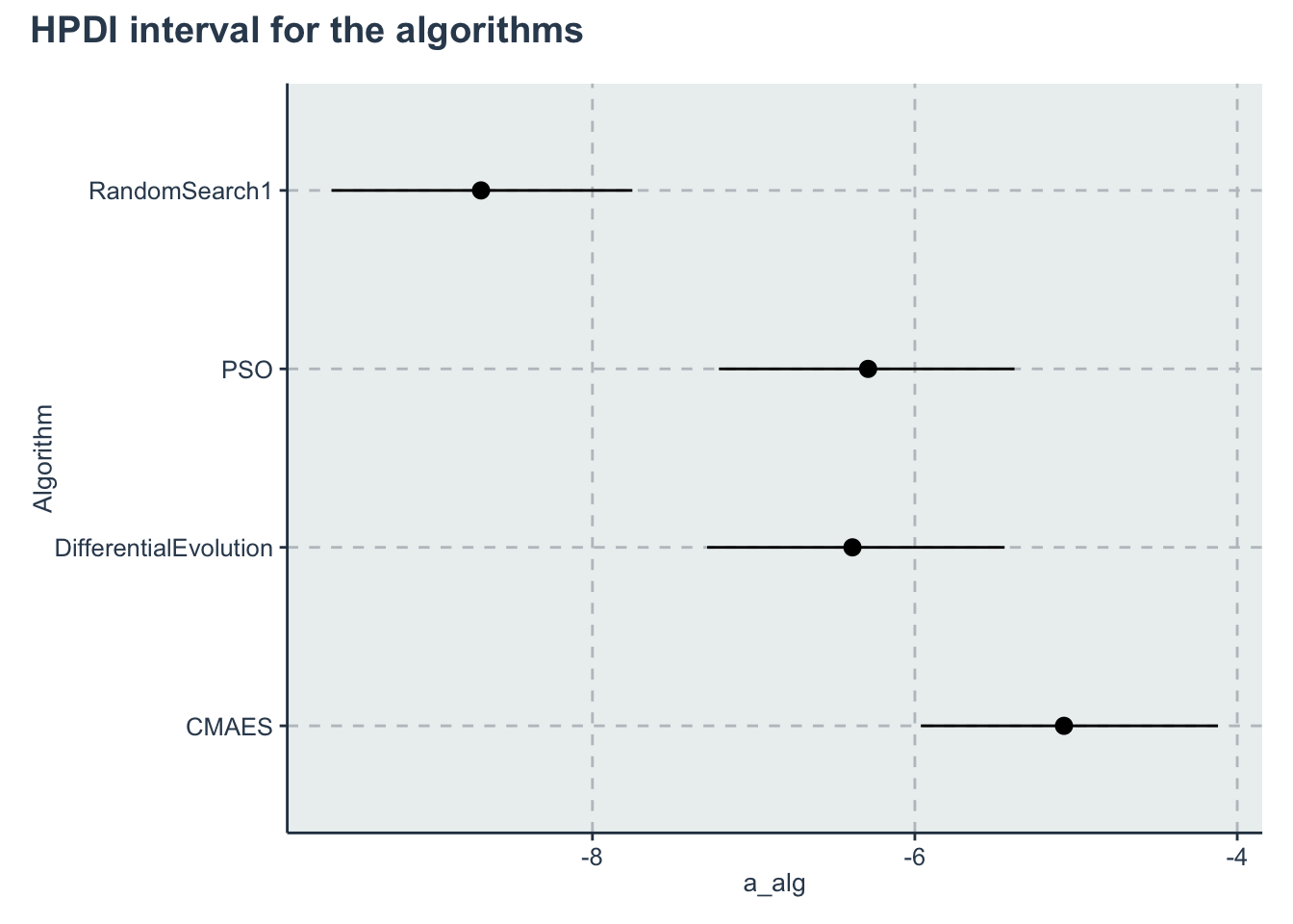

p_noise<-ggplot(data=hpdi_noise, aes(x=Parameter))+
  geom_pointrange(aes(
    ymin=HPDI.lower, 
    ymax=HPDI.higher, 
    y=Mean))+
  labs(y="b_noise", x="Algorithm")+
  coord_flip()
p_noise + plot_annotation(title = 'HPDI interval for noise coefficient')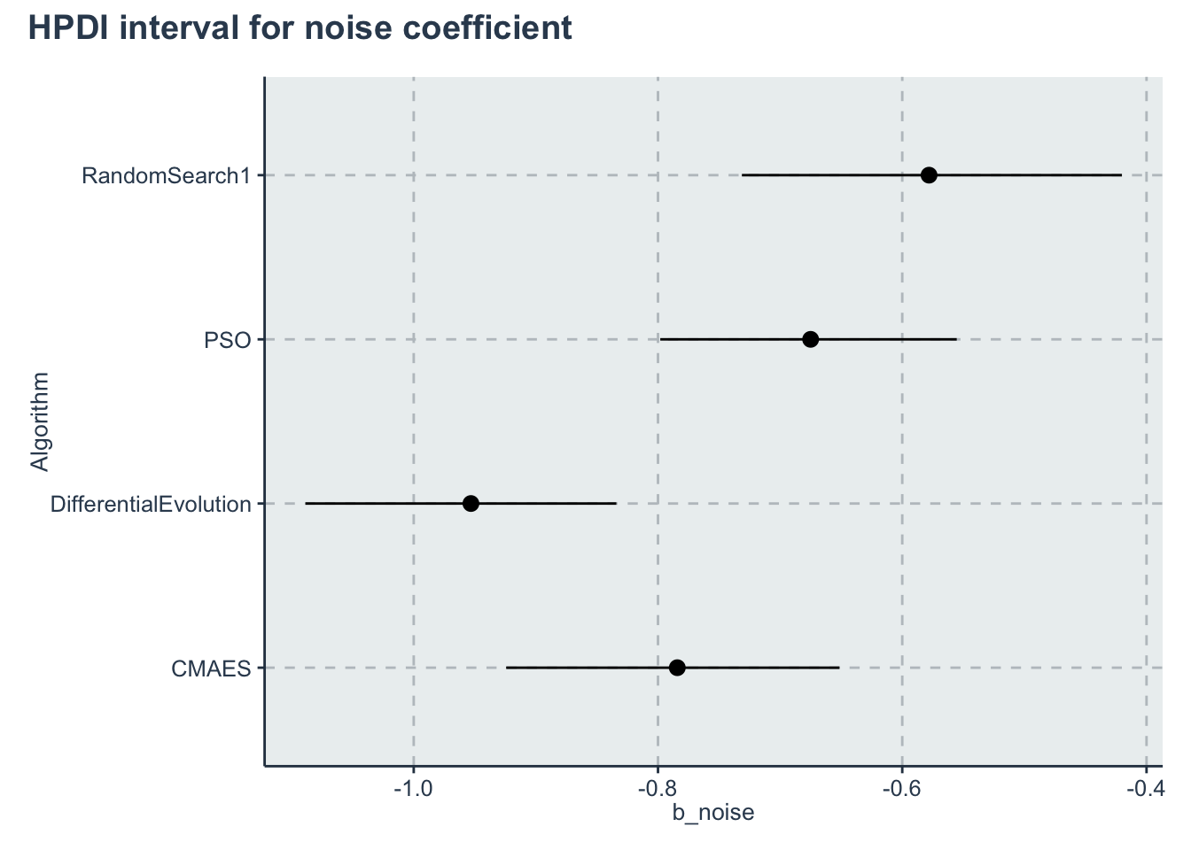

p_s <- ggplot(data=hpdi_s, aes(x=Parameter))+
  geom_pointrange(aes(
    ymin=HPDI.lower, 
    ymax=HPDI.higher, 
    y=Mean))+
  labs(y="Estimate of s", x="Parameter")+
  coord_flip()
p_s + plot_annotation(title = 'HPDI interval std of the benchmarks')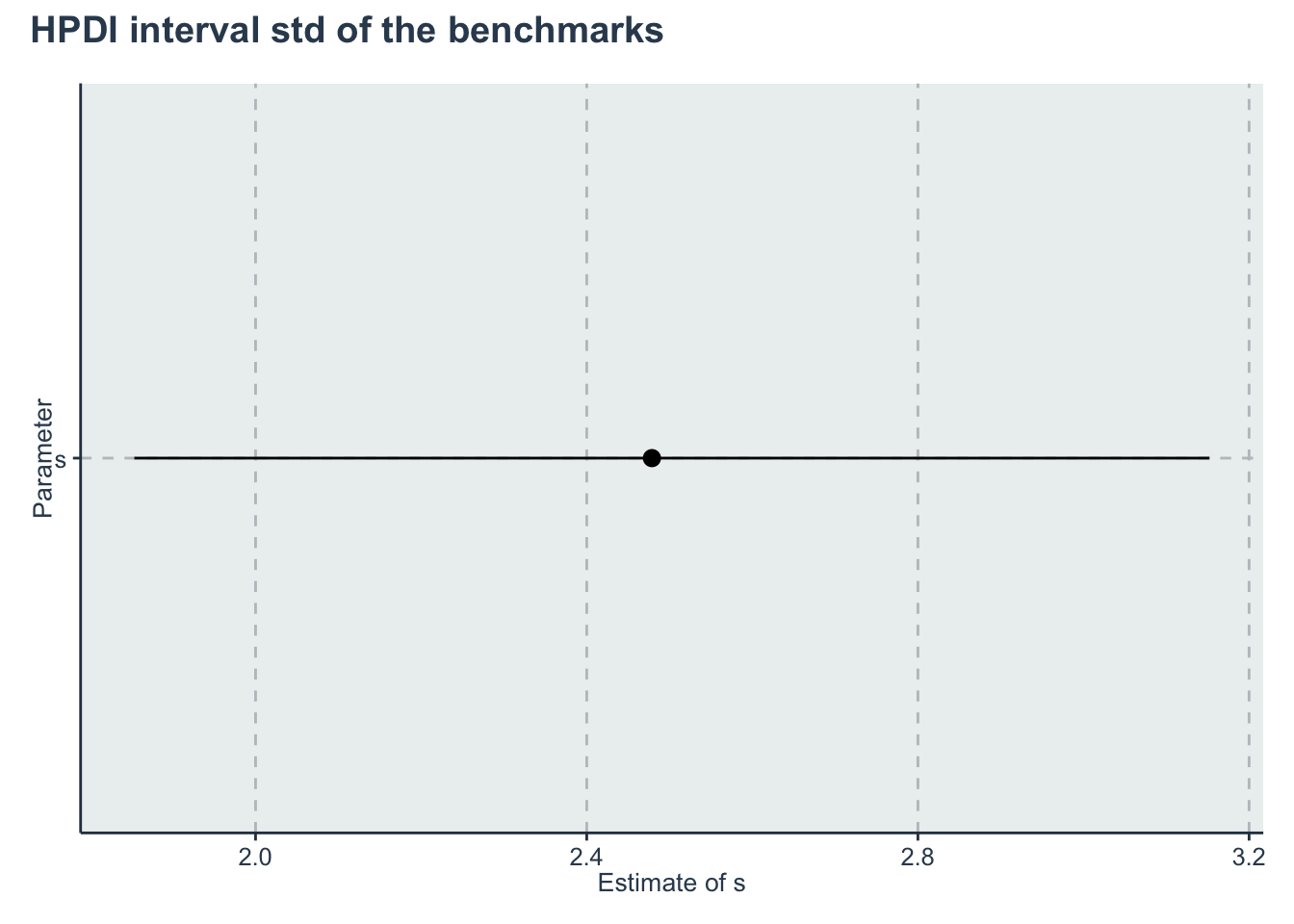

5.4.2 Hazard ratio

hr_table <- tibble(
  "Algorithms" = algorithms,
  "Baseline HR" = exp(hpdi_algorithm$Mean),
  "Noise HR" = exp(hpdi_noise$Mean))

kable(hr_table, booktabs=T, format.args = list(scientific = FALSE), digits = 3) %>% 
  kable_styling(bootstrap_options = c("striped", "hover", "condensed")) %>% 
  kableExtra::scroll_box(width = "100%")

Algorithms	Baseline HR	Noise HR
CMAES	0.006	0.456
DifferentialEvolution	0.002	0.386
PSO	0.002	0.509
RandomSearch1	0.000	0.561

5.4.3 Iterations to Converge

To obtain the average iteration to converge we first extract samples from the posterior distribution

Looking at the average value of the data regardless of the benchmarks

d_no_na <- d %>% drop_na(y)
d_no_na %>% group_by(Algorithm) %>% summarise(Mean=mean(y))

# A tibble: 4 x 2
  Algorithm               Mean
  <chr>                  <dbl>
1 CMAES                   115.
2 DifferentialEvolution  3340.
3 PSO                    2406.
4 RandomSearch1         13951.

posterior <- rstan::extract(timetoconverge_fit)
a <- as_tibble(posterior$a_alg)
colnames(a) <- algorithms

lambda <- exp(a)
mu <- 1/lambda


#Creating a HPD table
timetoconverge_table<-as_tibble(HDInterval::hdi(mu,credMass=0.95), rownames = "Metric") %>%
  tibble::add_row(Metric="Mean",CMAES=mean(mu$CMAES), DifferentialEvolution=mean(mu$DifferentialEvolution), PSO=mean(mu$PSO), RandomSearch1=mean(mu$RandomSearch1)) %>% 
  tidyr::pivot_longer(cols=-Metric,names_to = 'Algorithms', values_to='values') %>% 
  tidyr::pivot_wider(names_from =Metric , values_from=values) %>% 
  dplyr::rename(Mean=Mean,
                'HPD low' = lower,
                'HPD high' = upper) %>% 
  dplyr::relocate(Algorithms, Mean)

saveRDS(timetoconverge_table, './statscomp-paper/tables/datafortables/averagetimetoconverge.RDS')

5.4.4 Merging hazards and time to converge table

5.4.5 Parameter table

rename_pars <- c(paste(rep('a_',length(algorithms)),algorithms, sep = ""), paste(rep('b_',length(algorithms)),algorithms, sep = ""),'s')

t<-create_table_model(timetoconverge_fit, c(a_alg, b_noise, 's'), rename_pars)

colnames(t)<-c("Parameter", "Mean", "HPD low", "HPD high")
saveRDS(t,'./statscomp-paper/tables/datafortables/timetoconverge-hr-par-table.RDS')