Chapter 6 Multiple-group comparison

We present here the Stan version of the BEST (Bayesian Estimation Supersedes the t Test) from John K. Kruschke. We will consider the following research question

• RQ5: Is there a difference in the time taken per function evaluation between the PSO, the RandomSearch1 and the Differential Evolution algorithms?

6.1 RQ5 Data preparation

We start importing the dataset

dataset <- readr::read_csv('./data/statscomp.csv')

Filtering the data that we want and applying some transformations

d <- dataset %>% 
  dplyr::filter(
    OptimizationSuccessful==TRUE &
    (Algorithm=="PSO" | Algorithm=="RandomSearch1" | Algorithm=="DifferentialEvolution")) %>% 
  dplyr::select(Algorithm, CostFunction, TimeToComplete, simNumber, MaxFeval) %>% 
  dplyr::mutate(y=10000*TimeToComplete/MaxFeval,
                CostFunctionID=create_index(CostFunction),
                AlgorithmID=create_index(Algorithm)) %>% 
  dplyr::select(Algorithm, AlgorithmID, CostFunction, CostFunctionID, y,-simNumber, -MaxFeval)

algorithms<-get_index_names_as_array(d$Algorithm)
bm <- get_index_names_as_array(d$CostFunction)

The data should look like this:

kable(dplyr::sample_n(d,size=10), "html",booktabs=T, format.args = list(scientific = FALSE), digits = 3) %>% 
  kable_styling(bootstrap_options = c("striped", "hover", "condensed")) %>% 
  kableExtra::scroll_box(width = "100%")

Algorithm	AlgorithmID	CostFunction	CostFunctionID	y
DifferentialEvolution	1	WhitleyN6	28	2.950
DifferentialEvolution	1	ChenBird	2	1.813
PSO	2	Trefethen	25	0.541
DifferentialEvolution	1	WhitleyN6	28	2.957
RandomSearch1	3	DiscusN2	6	0.517
PSO	2	RosenbrockRotatedN6	14	1.747
RandomSearch1	3	Giunta	8	0.379
RandomSearch1	3	QingN2	13	0.190
RandomSearch1	3	Schwefel2d4N6	20	0.436
RandomSearch1	3	Damavandi	5	0.360

Some initial visualizations in terms of box-plots

p1<-ggplot(d) +
  geom_boxplot(aes(x=Algorithm, y=y))+
  labs(y="Time to complete x10,000 (s)")
p1 + plot_annotation(title ="Box-plot of the runtime per function evaluation")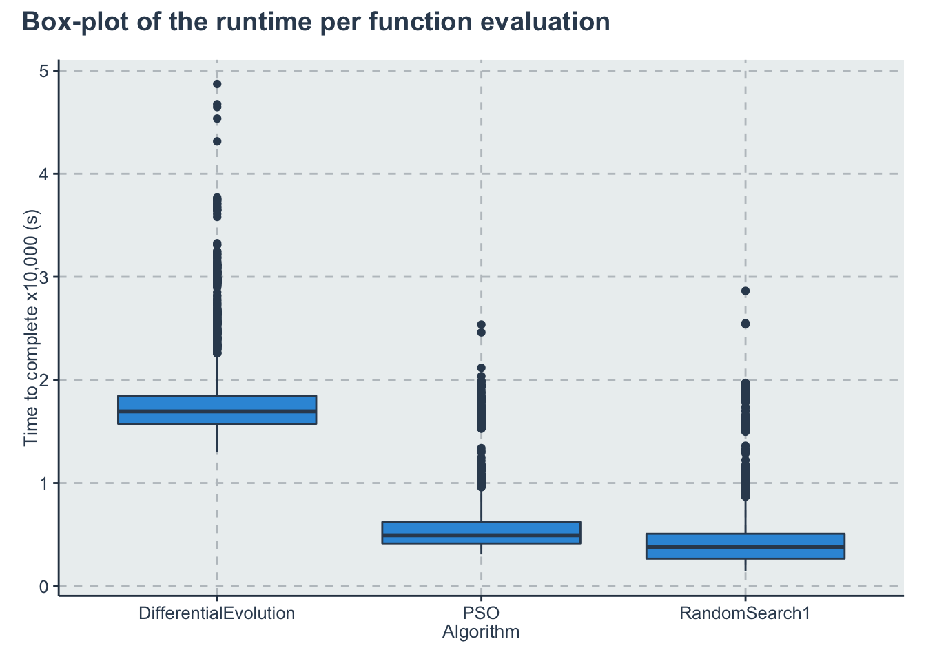

lmfit <- lm(y~Algorithm, data=d)

p2<-ggplot()+
  geom_qq(aes(sample=lmfit$residuals))+
  geom_qq_line(aes(sample=lmfit$residuals))+
  labs(x="Standard normal quantiles", y="Sample quantiles")
p2 + plot_annotation(title = "Q-Q plot for normality analysis")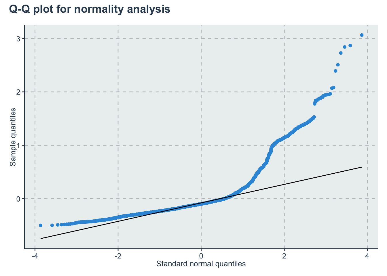

Verifying that the log of the runtime still present high tailed distributions

d2<-d
d2$y <- log(d2$y)
lmfit2 <- lm(y~Algorithm, data=d2)
p3<-ggplot()+
  geom_qq(aes(sample=lmfit2$residuals))+
  geom_qq_line(aes(sample=lmfit2$residuals))+
  labs(x="Standard normal quantiles", y="Sample quantiles")
p2 + plot_annotation(title = "Q-Q plot with the log of runtime")

6.2 RQ5 Stan model

The Stan model is specified in the file: './stanmodels/multiplegroups.stan'. Note that at the end of the model we commented the generated quantities. This block generates the predictive posterior y_rep and the log likelihood, log_lik. These values are useful in diagnosing and validating the model but the end file is extremely large (~1Gb for 2000 iterations) and make many of the following calculations slow. If the reader wants to see these values is just to uncomment and run the stan model again.

print_stan_code('./stanmodels/multiplegroups.stan')

// Multiple group comparison
// Author: David Issa Mattos
// Date: 23 June 2020
//
//

data {
 int <lower=1> N_total; // Sample size
 real y[N_total]; // time to complete variable

 //To model each algorithm independently
 int <lower=1> N_algorithm; // Number of algorithms
 int algorithm_id[N_total]; //vector that has the id of each algorithm
 
 //To model the influence of each benchmark
 int <lower=1> N_bm;
 int bm_id[N_total];
}

parameters {
  //Fixed effect
  real a_alg[N_algorithm];//the mean effect given by the algorithms
  real <lower=0> sigma[N_algorithm];//std for the student t

  // //Random effect. The effect of the benchmarks
  real a_bm_norm[N_bm];//the mean effect given by the base class type
  real<lower=0> s;//std for the random effects
  
  real<lower=0> nu;//std for the random effects
  
}

model {
  real mu[N_total];
  real sigma_i[N_total];

  sigma ~ exponential(1);
  nu ~ exponential(1.0/30.0);
  
  //Fixed effect
  a_alg ~ normal(0,1);
  
  // //Random effects
  s ~ exponential(1);
  a_bm_norm ~ normal(0,1);

  for (i in 1:N_total)
  {
    
     mu[i] = a_alg[algorithm_id[i]] + a_bm_norm[bm_id[i]]*s;
     sigma_i[i] = sigma[algorithm_id[i]];
  }
  
  y ~ student_t(nu, mu, sigma_i);
}

//Uncoment this part to get the posterior predictives and the log likelihood
//But note that it takes a lot of space in the final model
// generated quantities{
//   vector [N_total] y_rep;
//   vector[N_total] log_lik;
//   for (i in 1:N_total){
//     real mu;
//     real sigma_i;
//     mu = a_alg[algorithm_id[i]] + a_bm_norm[bm_id[i]]*s;
//     sigma_i = sigma[algorithm_id[i]];
//     y_rep[i] = student_t_rng(nu,mu,sigma_i);
//     
//     //Log likelihood
//     log_lik[i] = student_t_lpdf(y[i] | nu,mu,sigma_i);
//     
//   }
// }

Let’s compile and start sampling with the Stan function. In the data folder you can find the specific data used to fit the model after all transformations "./data/multiplegroup-data.RDS"

standata <- list(
  N_total=nrow(d),
  y = d$y,
  N_algorithm = length(algorithms),
  algorithm_id = d$AlgorithmID,
  N_bm = length(bm),
  bm_id = d$CostFunctionID
  )
saveRDS(standata, file = "./data/multiplegroups-data.RDS")

For computation time sake we are not running this chunk every time we compile this document. From now on we will load from the saved Stan fit object. However, when we change our model or the data we can just run this chunk separately. Here we increased the maxtreedepth and the number of iterations so we have a higher effective sample for inference. Both of these do not impact the validity of the chain just the computation efficiency.

standata<-readRDS("./data/multiplegroups-data.RDS")
multiplegroup_fit <- stan(file = './stanmodels/multiplegroups.stan',
                     data=standata,
                     chains = 4,
                     warmup = 400,
                     iter = 4000,
                     control = list(max_treedepth = 15))
saveRDS(multiplegroup_fit, file = "./data/multiplegroups-fit.RDS")

6.3 RQ5 Diagnosis

a_alg_v <- c("a_alg[1]",
           "a_alg[2]",
           "a_alg[3]")

sigma_v <- c("sigma[1]",
           "sigma[2]",
           "sigma[3]")
rstan::traceplot(multiplegroup_fit, pars=a_alg_v)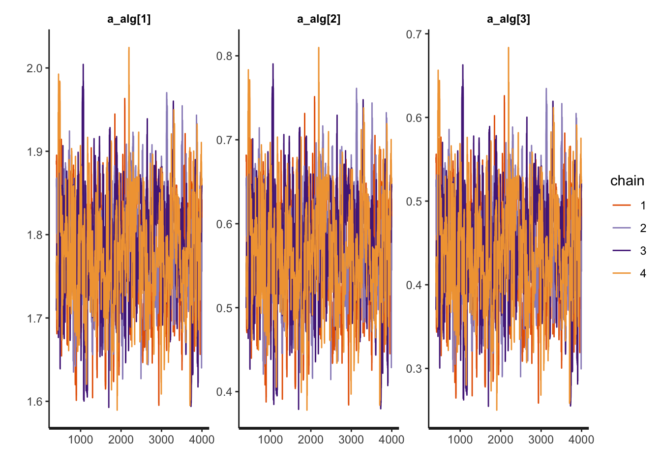

rstan::traceplot(multiplegroup_fit, pars=sigma_v)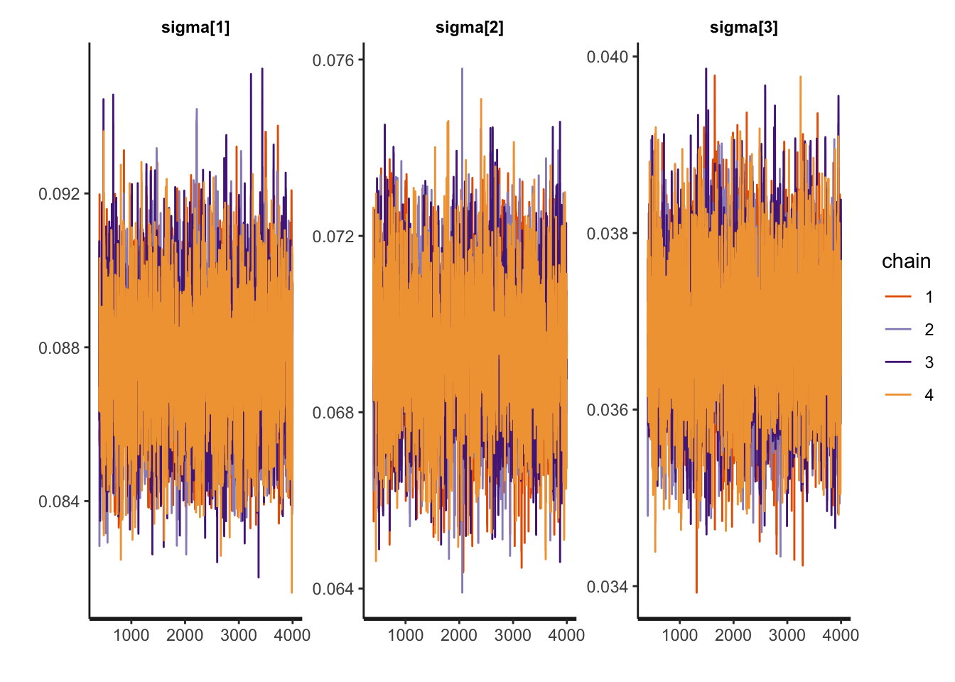

rstan::traceplot(multiplegroup_fit, pars=c('s', 'nu'))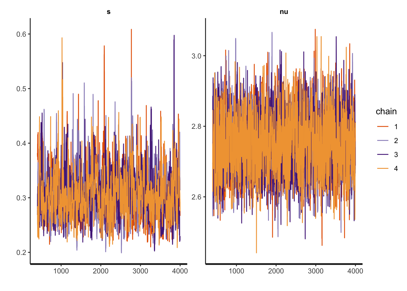

Another diagnosis is to look at the Rhat. If Rhat is greater than 1.05 it indicates a divergence in the chains (they did not mix well). The table below shows a summary of the sampling.

kable(summary(multiplegroup_fit)$summary, "html",) %>% 
  kable_styling(bootstrap_options = c('striped',"hover", "condensed" )) %>% 
  kableExtra::scroll_box(width = "100%")

	mean	se_mean	sd	2.5%	25%	50%	75%	97.5%	n_eff	Rhat
a_alg[1]	1.7811268	0.0026230	0.0606078	1.6619826	1.7403893	1.7820330	1.8215807	1.8982458	533.8817	1.006126
a_alg[2]	0.5691139	0.0026209	0.0605588	0.4496716	0.5283954	0.5700587	0.6093643	0.6855433	533.8829	1.006094
a_alg[3]	0.4423529	0.0026208	0.0605582	0.3233317	0.4013482	0.4432400	0.4826083	0.5580626	533.9264	1.006091
sigma[1]	0.0877444	0.0000318	0.0017455	0.0843878	0.0865374	0.0877212	0.0889341	0.0911437	3011.1145	1.001623
sigma[2]	0.0694441	0.0000277	0.0015140	0.0664710	0.0684330	0.0694499	0.0704463	0.0724822	2976.8074	1.000836
sigma[3]	0.0368688	0.0000144	0.0008039	0.0352959	0.0363257	0.0368479	0.0374083	0.0384708	3121.5824	1.000719
a_bm_norm[1]	0.7169454	0.0087107	0.2135654	0.2988931	0.5710651	0.7142151	0.8674880	1.1328629	601.1139	1.008025
a_bm_norm[2]	-0.1824269	0.0085491	0.1988784	-0.5714764	-0.3176881	-0.1827604	-0.0451221	0.1940826	541.1669	1.005750
a_bm_norm[3]	-0.5830931	0.0091159	0.2163121	-1.0160424	-0.7275807	-0.5801526	-0.4404438	-0.1643768	563.0722	1.003927
a_bm_norm[4]	-0.6091954	0.0091666	0.2178293	-1.0467759	-0.7534750	-0.6062762	-0.4656718	-0.1855039	564.6959	1.003882
a_bm_norm[5]	-0.2485564	0.0086165	0.2008707	-0.6432752	-0.3856466	-0.2485221	-0.1111202	0.1316417	543.4600	1.005561
a_bm_norm[6]	0.4734111	0.0084824	0.2024756	0.0780666	0.3334823	0.4720095	0.6152515	0.8568556	569.7825	1.007887
a_bm_norm[7]	-0.6423130	0.0092312	0.2198717	-1.0846795	-0.7887968	-0.6386941	-0.4972334	-0.2139691	567.3092	1.003799
a_bm_norm[8]	-0.1644817	0.0085326	0.1985217	-0.5517190	-0.2996106	-0.1657384	-0.0275923	0.2129775	541.3154	1.005963
a_bm_norm[9]	2.1116300	0.0121812	0.3393819	1.4484849	1.8816608	2.1092589	2.3358436	2.7967160	776.2394	1.005745
a_bm_norm[10]	-0.1812781	0.0085416	0.1989285	-0.5714155	-0.3176169	-0.1816472	-0.0444326	0.1975518	542.3993	1.005821
a_bm_norm[11]	0.9019238	0.0089863	0.2249558	0.4576177	0.7501431	0.8991386	1.0577316	1.3417398	626.6611	1.007809
a_bm_norm[12]	-0.7818005	0.0095262	0.2292960	-1.2427092	-0.9348107	-0.7782093	-0.6287008	-0.3328971	579.3611	1.003212
a_bm_norm[13]	-0.6775106	0.0092827	0.2220651	-1.1227791	-0.8255683	-0.6734795	-0.5296425	-0.2434466	572.2849	1.003527
a_bm_norm[14]	1.7137941	0.0109291	0.2967903	1.1337453	1.5123317	1.7108835	1.9123530	2.3102016	737.4474	1.006425
a_bm_norm[15]	-0.2518458	0.0086224	0.2009569	-0.6477380	-0.3884656	-0.2520031	-0.1136934	0.1301903	543.1896	1.005519
a_bm_norm[16]	-0.6890408	0.0093176	0.2228297	-1.1395233	-0.8382348	-0.6855899	-0.5409571	-0.2539657	571.9248	1.003543
a_bm_norm[17]	-0.2997380	0.0086702	0.2027220	-0.6996320	-0.4386068	-0.2983614	-0.1626570	0.0871212	546.6910	1.005343
a_bm_norm[18]	-0.2065718	0.0085791	0.1997227	-0.5978602	-0.3420286	-0.2057953	-0.0687583	0.1743771	541.9588	1.005684
a_bm_norm[19]	-0.1781351	0.0085411	0.1988323	-0.5689114	-0.3141829	-0.1783365	-0.0407893	0.1991033	541.9402	1.005823
a_bm_norm[20]	0.0013479	0.0084299	0.1959243	-0.3801857	-0.1321950	-0.0011718	0.1384331	0.3748182	540.1669	1.006703
a_bm_norm[21]	-0.0381568	0.0084334	0.1961037	-0.4215247	-0.1727083	-0.0400992	0.0998043	0.3345669	540.7160	1.006430
a_bm_norm[22]	-0.2591012	0.0086473	0.2014404	-0.6537203	-0.3957154	-0.2589614	-0.1220667	0.1262415	542.6678	1.005472
a_bm_norm[23]	-0.7358550	0.0094254	0.2260798	-1.1892931	-0.8858307	-0.7320868	-0.5846833	-0.2939862	575.3385	1.003330
a_bm_norm[24]	-0.8254234	0.0096072	0.2324392	-1.2935835	-0.9805076	-0.8213645	-0.6689679	-0.3684101	585.3639	1.003067
a_bm_norm[25]	-0.3366898	0.0087284	0.2039811	-0.7369234	-0.4748569	-0.3359966	-0.1992994	0.0536531	546.1521	1.005150
a_bm_norm[26]	0.3488281	0.0084028	0.1985740	-0.0350128	0.2120805	0.3487199	0.4879435	0.7238281	558.4606	1.007803
a_bm_norm[27]	-0.7346498	0.0094058	0.2258222	-1.1905483	-0.8847851	-0.7302798	-0.5839647	-0.2927947	576.4249	1.003359
a_bm_norm[28]	3.6998131	0.0182556	0.5324392	2.6893552	3.3338793	3.6905820	4.0513884	4.7696181	850.6446	1.004008
a_bm_norm[29]	-0.4143554	0.0088376	0.2074474	-0.8239239	-0.5542043	-0.4118008	-0.2764703	-0.0164877	550.9920	1.004714
a_bm_norm[30]	-0.1770084	0.0085576	0.1989495	-0.5672901	-0.3128015	-0.1772755	-0.0397254	0.2004904	540.4818	1.005940
s	0.3072466	0.0014798	0.0441124	0.2352709	0.2768578	0.3021747	0.3322788	0.4069552	888.6323	1.001588
nu	2.7532026	0.0015421	0.0802559	2.6021136	2.6972495	2.7520588	2.8075206	2.9112477	2708.6351	1.001055
lp__	14070.2753067	0.1671716	5.9172571	14057.6082046	14066.4863632	14070.6208015	14074.4422447	14080.7870357	1252.8982	1.000465

6.4 RQ5 Results and Plots

First lets get the HPDI of every parameter.

Then we restrict to the algorithms, them to the slopes, then to the parameter s

hpdi <- get_HPDI_from_stanfit(multiplegroup_fit)

hpdi_algorithm <- hpdi %>% 
      dplyr::filter(str_detect(Parameter, "a_alg\\[")) %>%
      dplyr::mutate(Parameter=algorithms) #Changing to the algorithms labels

hpdi_sigma<- hpdi %>% 
      dplyr::filter(str_detect(Parameter, "sigma\\[")) %>%
      dplyr::mutate(Parameter=algorithms) #Changing to the algorithms labels

hpdi_s <- hpdi %>% 
      dplyr::filter(Parameter=='s')


hpdi_nu <- hpdi %>% 
      dplyr::filter(Parameter=='nu')


hpdi_nu_s <- hpdi %>% 
      dplyr::filter(Parameter=='nu' | Parameter=='s')

p_alg<-ggplot(data=hpdi_algorithm, aes(x=Parameter))+
  geom_pointrange(aes(
    ymin=HPDI.lower, 
    ymax=HPDI.higher, 
    y=Mean))+
  labs(y="a_alg", x="Algorithm")+
  theme(axis.title.x= element_blank())+
  coord_flip()
p_alg + plot_annotation(title = 'HPDI interval for the algorithms')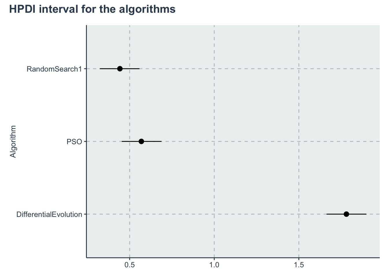

p_sigma<-ggplot(data=hpdi_sigma, aes(x=Parameter))+
  geom_pointrange(aes(
    ymin=HPDI.lower, 
    ymax=HPDI.higher, 
    y=Mean))+
  labs(y="sigma", x="Algorithm")+
  theme(axis.title.x= element_blank())+
  coord_flip()
p_sigma + plot_annotation(title = 'HPDI interval for sigma')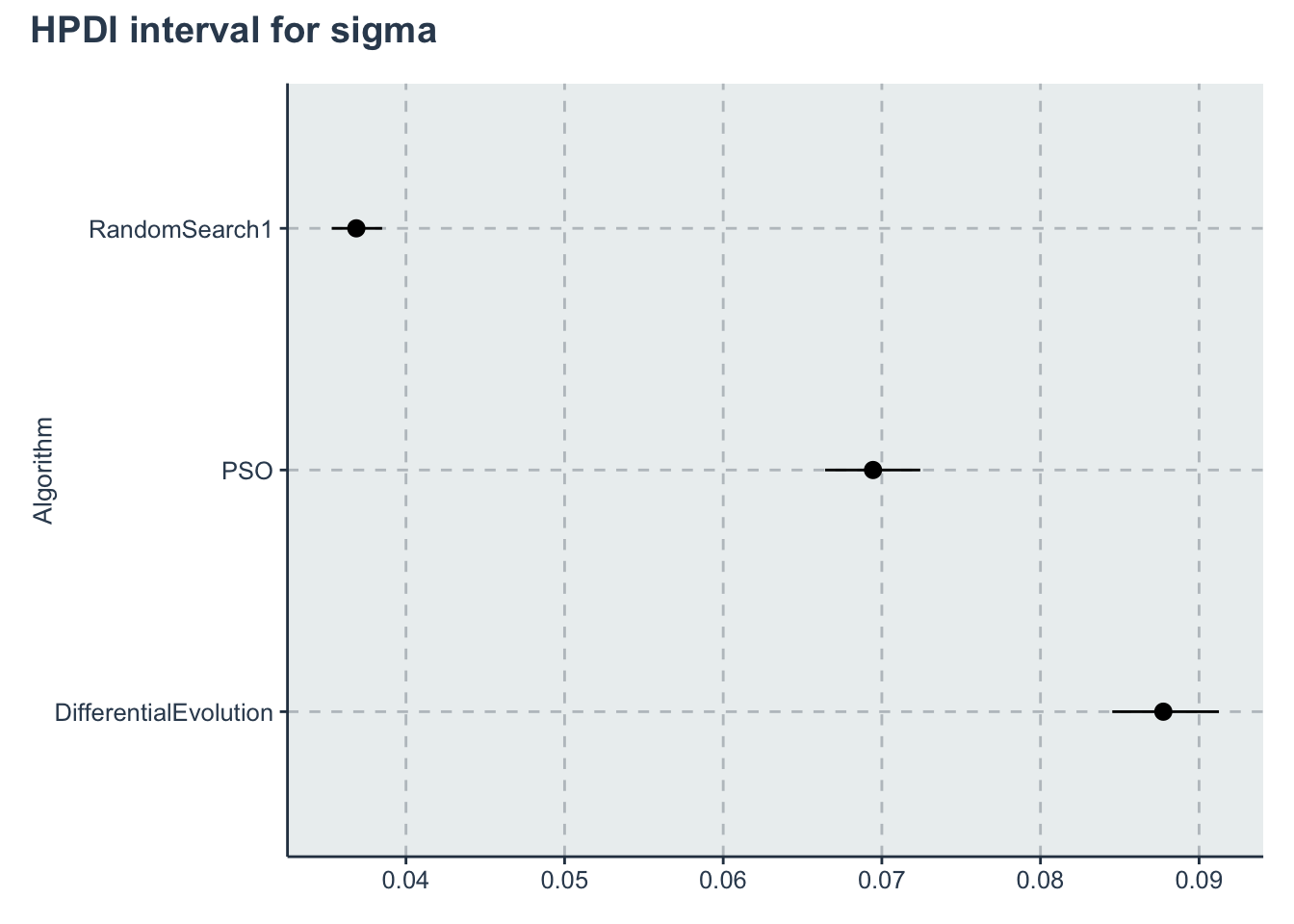

p_s <- ggplot(data=hpdi_s, aes(x=Parameter))+
  geom_pointrange(aes(
    ymin=HPDI.lower, 
    ymax=HPDI.higher, 
    y=Mean))+
  labs(y="s", x="Parameter")+
  coord_flip()
p_s + plot_annotation(title = 'HPDI interval std of the benchmarks')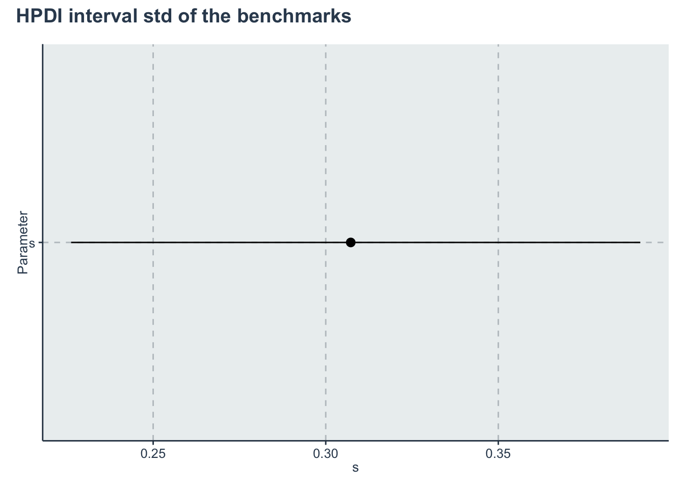

p_nu <- ggplot(data=hpdi_nu, aes(x=Parameter))+
  geom_pointrange(aes(
    ymin=HPDI.lower, 
    ymax=HPDI.higher, 
    y=Mean))+
  labs(y="nu", x="Parameter")+
  coord_flip()
p_nu + plot_annotation(title = 'HPDI interval of the degree of freedom')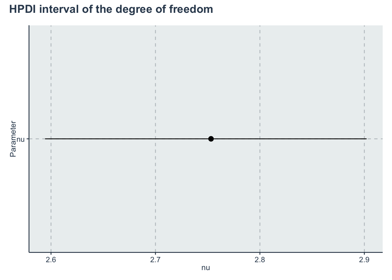

p_nu_s <- ggplot(data=hpdi_nu_s, aes(x=Parameter))+
  geom_pointrange(aes(
    ymin=HPDI.lower, 
    ymax=HPDI.higher, 
    y=Mean))+
  labs(y="Estimate of s and nu", x="Parameter")+
  theme(axis.title.x= element_blank())+
  coord_flip()

p_nu_s + plot_annotation(title = 'HPDI interval')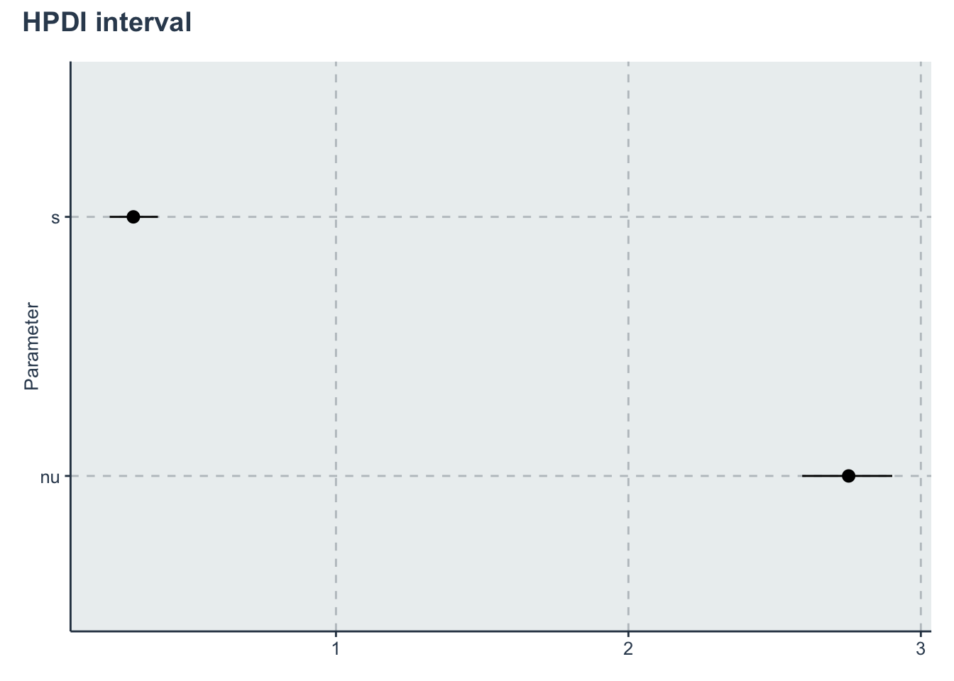

Now lets get a posterior distribution of the difference

posterior <- rstan::extract(multiplegroup_fit)
a_alg <- as_tibble(posterior$a_alg)
colnames(a_alg) <- algorithms
sample_a_alg <- dplyr::sample_n(a_alg, size=1000, replace=T) %>% 
  dplyr::mutate(PSO_Random = PSO-RandomSearch1,
                DE_PSO= DifferentialEvolution-PSO,
                DE_Random = DifferentialEvolution-RandomSearch1) %>% 
  dplyr::select(-DifferentialEvolution,-PSO,-RandomSearch1)

#Getting HPDI from a data frame and creating a table instead of plotting...
hpdi_diff<-HDInterval::hdi(sample_a_alg,credMass=0.95)
hpdi_diff<-hpdi_diff %>% as_tibble(rownames = "Metric") %>% 
  tibble::add_row(Metric="Mean", PSO_Random=mean(sample_a_alg$PSO_Random), DE_PSO=mean(sample_a_alg$DE_PSO), DE_Random=mean(sample_a_alg$DE_Random)) %>%
  tidyr::pivot_longer(cols=-Metric, names_to="AlgorithmDifference", values_to='values') %>% 
  tidyr::pivot_wider(names_from =Metric , values_from=values) %>% 
  dplyr::mutate(Difference=c('PSO - RandomSearch', 'DiffEvolution - PSO', 'DiffEvolution - RandomSearch')) %>% 
  dplyr::select(Difference, Lower=lower, Mean, Upper=upper)

kable(hpdi_diff, booktabs=T, format.args = list(scientific = FALSE), digits = 3) %>% 
  kable_styling(bootstrap_options = c("striped", "hover", "condensed")) %>% 
  kableExtra::scroll_box(width = "100%")

Difference	Lower	Mean	Upper
PSO - RandomSearch	0.123	0.127	0.130
DiffEvolution - PSO	1.207	1.212	1.217
DiffEvolution - RandomSearch	1.334	1.339	1.343

Creating an output table

rename_pars <- c(
  paste(rep('a_',length(algorithms)),algorithms, sep = ""),
  paste(rep('sigma_',length(algorithms)),algorithms, sep = ""),
  's',
  'nu')
t<-create_table_model(multiplegroup_fit, pars=c(a_alg_v, sigma_v, 's','nu'),rename_pars)
colnames(t)<-c("Parameter", "Mean", "HPD low", "HPD high")
saveRDS(t,'./statscomp-paper/tables/datafortables/multiplegroupsdifference-par-table.RDS')