Chapter 7 Extra II: PBO 625 dimensions | Online appendix for the paper: “On the Assessment of Benchmark Suites for Algorithm Comparison”

7.1 Importing the data

To illustrate and make the analysis we will use 5 as the number of dimensions for the benchmark functions

d_pbo <- read_csv('data/pbo.csv') %>% 
  select(algId, DIM, funcId, runs, succ, budget) %>% 
  filter(DIM==625) %>%
  mutate(algId_index = as.integer(as.factor(algId)))

#vector with the names in order
benchmarks <- seq(1,23)
algorithms <- levels(as.factor(d_pbo$algId))

7.2 Preparing the Stan data

pbo_standata <- list(
  N = nrow(d_pbo),
  y_succ = as.integer(d_pbo$succ),
  N_tries = as.integer(d_pbo$runs),
  p = d_pbo$algId_index,
  Np = as.integer(length(unique(d_pbo$algId_index))),
  item = as.integer(d_pbo$funcId),
  Nitem = as.integer(length(unique(d_pbo$funcId)))
)

irt2pl <- cmdstan_model('models/irt2pl.stan') 
fit_pbo <- irt2pl$sample(
  data= pbo_standata,
  seed = seed,
  chains = 4,
  iter_sampling = 4000,
  parallel_chains = 4,
  max_treedepth = 15
)
fit_pbo$save_object(file='fitted/pbo625.RDS')

To load the fitted model to save time in compiling this document

fit_pbo<-readRDS('fitted/pbo625.RDS')

7.3 Diagnostics

Getting the draws from the posterior

draws_a <- fit_pbo$draws('a')
draws_b <- fit_pbo$draws('b')
draws_theta <- fit_pbo$draws('theta')

7.3.1 Traceplots

mcmc_trace(draws_a)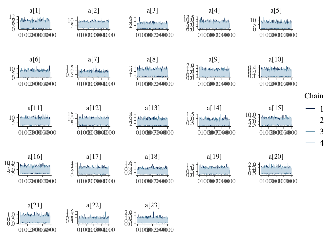

mcmc_trace(draws_b)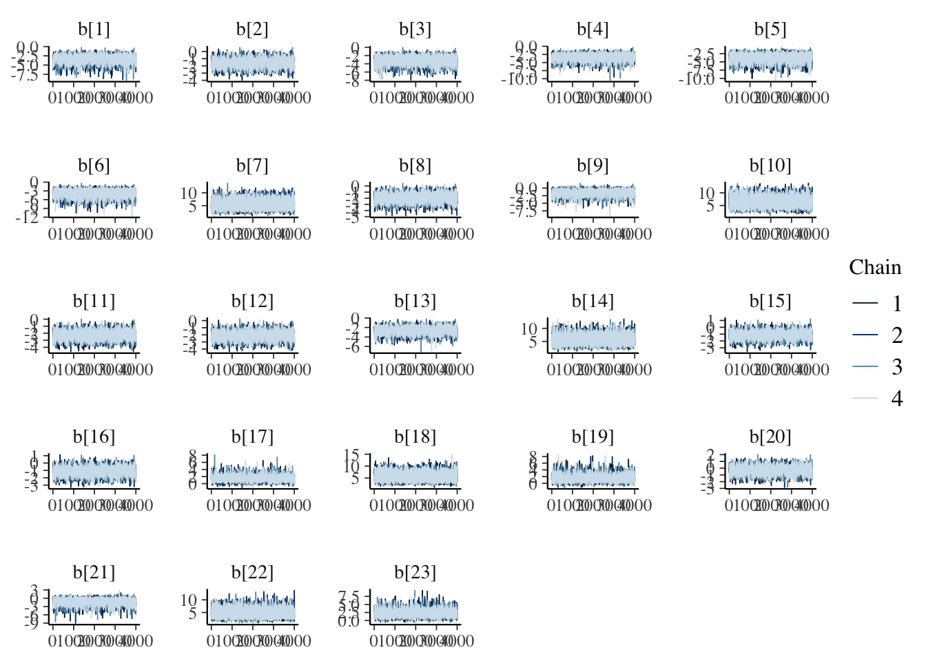

mcmc_trace(draws_theta)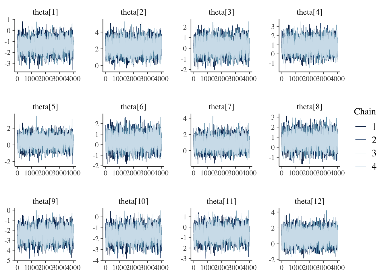

7.4 Results

fit_summary_a_b <- fit_pbo$summary(c('a','b'))
fit_summary_a <- fit_pbo$summary(c('a'))
fit_summary_b <- fit_pbo$summary(c('b'))
fit_summary_theta <- fit_pbo$summary(c('theta'))

7.4.1 Difficulty and discrimination

Table for the benchmark functions

table_benchmarks <- fit_summary_a_b %>% 
  select('Benchmark ID'=variable, 
         Median=median,
         'CI 5%'=q5,
         'CI 95%'=q95)

table_benchmarks$'Benchmark ID'<-rep(benchmarks,2)

kable(table_benchmarks,
      caption='Summary values of the discrimination and difficulty level parameters for the PBO benchmarks', 
      booktabs=T,
      digits =3,
      format='html',
      linesep = "") %>% 
  kable_styling() %>% 
  pack_rows("Discrimination value (a)",1,23) %>% 
  pack_rows("Difficulty level (b)",23,46)

Table 7.1: Summary values of the discrimination and difficulty level parameters for the PBO benchmarks
Benchmark ID	Median	CI 5%	CI 95%
Discrimination value (a)
1	2.919	1.210	6.017
2	4.455	2.635	7.121
3	1.431	0.775	2.507
4	2.936	1.199	6.089
5	2.693	1.115	5.857
6	2.679	1.095	5.898
7	0.425	0.258	0.709
8	1.402	0.875	2.193
9	0.596	0.271	1.050
10	0.160	0.098	0.259
11	4.982	2.801	8.026
12	5.966	3.669	9.031
13	2.267	1.229	3.941
14	0.429	0.261	0.713
15	4.119	2.726	6.184
16	4.124	2.717	6.154
17	1.154	0.507	2.025
18	0.430	0.261	0.714
19	0.474	0.204	0.851
20	0.833	0.506	1.272
21	0.387	0.149	0.698
22	0.355	0.207	0.605
Difficulty level (b)
23	0.507	0.250	0.873
1	-3.133	-4.765	-1.961
2	-1.601	-2.543	-0.650
3	-3.031	-4.616	-1.801
4	-3.133	-4.780	-1.973
5	-3.522	-5.524	-2.213
6	-3.531	-5.666	-2.218
7	5.279	3.149	8.293
8	-1.929	-3.020	-0.898
9	-1.334	-2.901	-0.219
10	6.256	3.759	9.466
11	-2.276	-3.269	-1.288
12	-2.132	-3.109	-1.159
13	-2.599	-3.765	-1.529
14	5.439	3.279	8.445
15	-1.146	-2.068	-0.220
16	-1.142	-2.083	-0.220
17	1.434	0.381	2.766
18	5.402	3.274	8.395
19	1.347	0.176	3.052
20	-0.323	-1.295	0.624
21	-1.083	-2.847	0.136
22	4.730	2.659	7.668
23	2.017	0.748	3.890

mcmc_intervals(draws_a) +
  scale_y_discrete(labels=benchmarks)+
  labs(x='Discrimination parameter (a)',
       y='Benchmark function ID',
       title='Discrimination parameter distribution (PBO)')

## Scale for 'y' is already present. Adding another scale for 'y', which will
## replace the existing scale.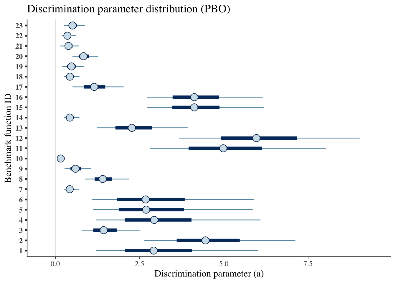

mcmc_intervals(draws_b) +
  scale_y_discrete(labels=benchmarks)+
  labs(x='Difficulty level parameter (b)',
       y='Benchmark function ID',
       title='Difficulty level parameter distribution (PBO)')

## Scale for 'y' is already present. Adding another scale for 'y', which will
## replace the existing scale.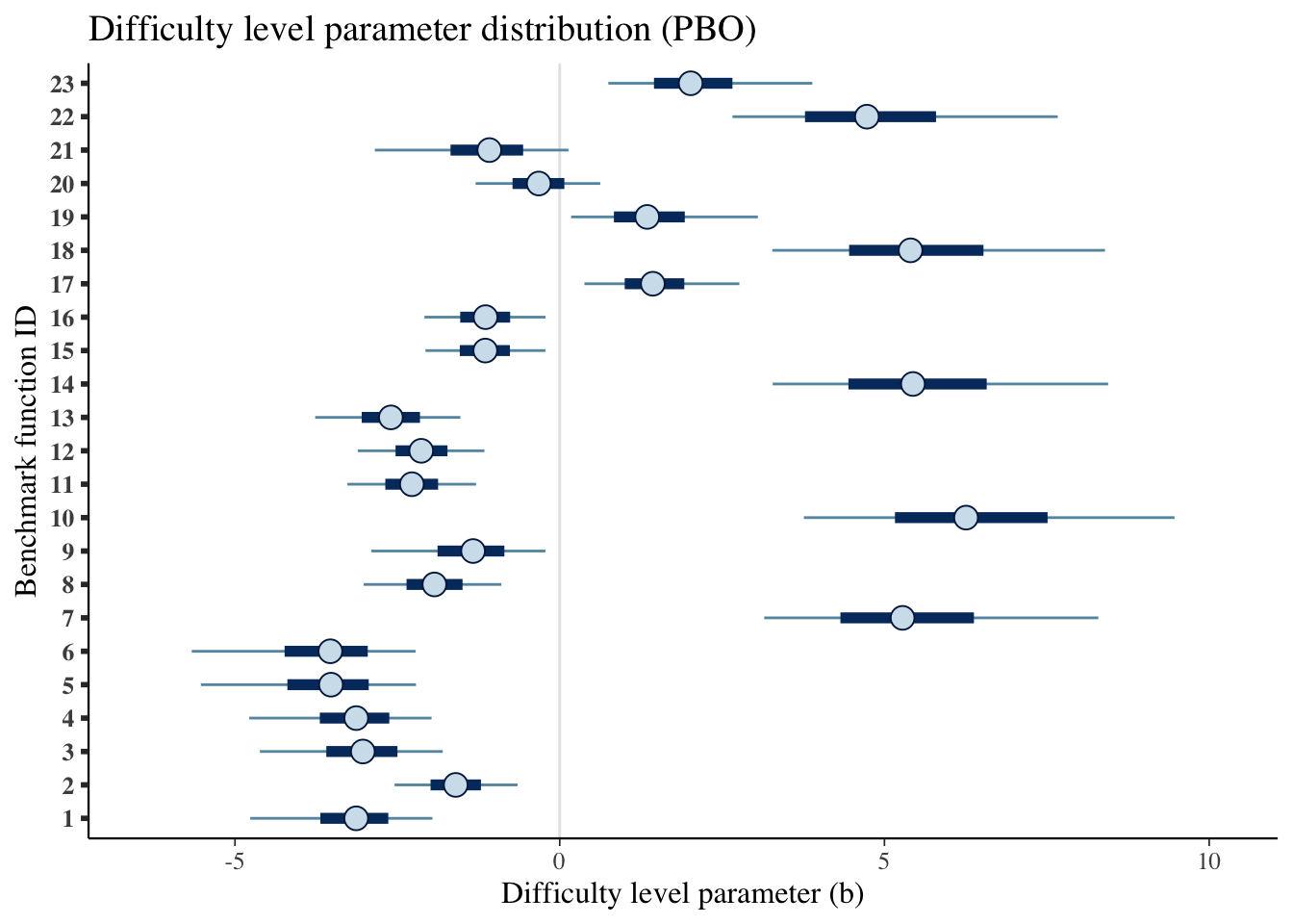

7.4.2 Ability

Creating a table

table_algorithms <- fit_summary_theta %>% 
  select(Algorithms=variable, 
         Median=median,
         'CI 5%'=q5,
         'CI 95%'=q95)

table_algorithms$Algorithms <- algorithms

kable(table_algorithms,
      caption='Summary values of the ability level of the algorithms (PBO)', 
      booktabs=T,
      digits =3,
      format='html',
      linesep = "") %>% 
  kable_styling()

Table 7.2: Summary values of the ability level of the algorithms (PBO)
Algorithms	Median	CI 5%	CI 95%
(1+(λ,λ)) GA	-1.371	-2.306	-0.437
(1+1) EA_>0	2.184	1.027	3.383
(1+1) fGA	0.139	-0.831	1.150
(1+10) EA_{r/2,2r}	0.865	-0.177	1.949
(1+10) EA_>0	0.340	-0.634	1.346
(1+10) EA_logNormal	0.330	-0.652	1.345
(1+10) EA_normalized	0.853	-0.177	1.926
(1+10) EA_var_ctrl	0.625	-0.384	1.709
(30,30) vGA	-2.402	-3.382	-1.426
EDA	-1.643	-2.587	-0.694
gHC	-0.629	-1.557	0.302
RLS	0.935	-0.312	2.158

mcmc_intervals(draws_theta) +
  scale_y_discrete(labels=algorithms)+
  labs(x=unname(TeX("Ability level ($\\theta$)")),
       y='Algorithm',
       title='Ability level parameter distribution (PBO)')

## Scale for 'y' is already present. Adding another scale for 'y', which will
## replace the existing scale.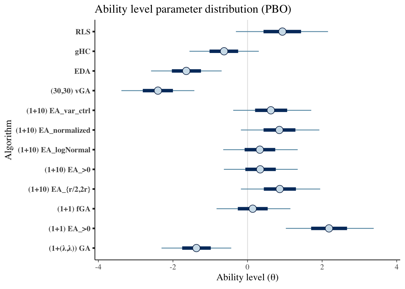

7.4.3 Item information

We will use the same functions from the BBOB case study

Creating a single data frame

item_information_df <- NULL
for(i in seq(1:length(benchmarks))){
  a<-as.matrix(fit_summary_a[i,c(3,6,7)])
  b<-as.matrix(fit_summary_b[i,c(3,6,7)])
  iinfo <- item_info_with_intervals(a=a,b=b,item = i,thetamin = -7, thetamax = 5)
  item_information_df <- rbind(item_information_df,iinfo)
}

Now we can create an information plot for every item

item_information_df %>% 
  pivot_wider(names_from = 'pars', values_from = 'Information') %>% 
  ggplot(aes(x=theta))+
    geom_line(aes(y=median), color='black')+
    # geom_line(aes(y=q05), color='red', linetype='dashed')+
    # geom_line(aes(y=q95), color='blue', linetype='dashed')+
    facet_wrap(~item,
               ncol=4) +
    labs(title='Item information curve (PBO)',
         x=unname(TeX("Ability ($\\theta$)")),
         y='Information',
         color='Information interval')+
    theme_bw() +
    theme(legend.position = 'bottom')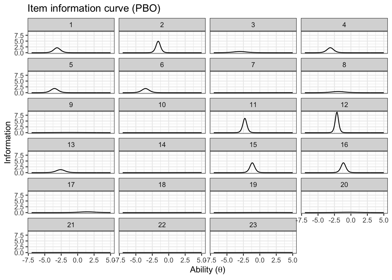

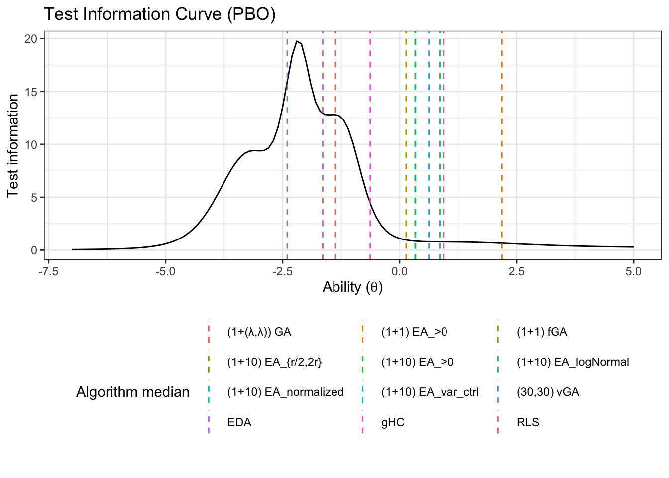
7.4.4 Test information

We can also look at the test information. First, we need to pivot wider so we can sum the items

test_information_df <- item_information_df %>% 
  pivot_wider(names_from = 'item', values_from = 'Information') %>% 
  mutate(TestInfo = dplyr::select(., -theta, -pars) %>% rowSums()) %>% 
  dplyr::select(theta, pars, TestInfo)

Now that we have calculated the test parameters we can plot the test information

First let’s get a horizontal line to show where the algorithms median ability lies

alg_median <- fit_summary_theta %>% 
  mutate(Algorithm=algorithms) %>% 
  select(Algorithm, median)

test_information_df %>% 
  dplyr::select(theta, pars, TestInfo) %>% 
  pivot_wider(names_from = 'pars', values_from = 'TestInfo') %>% 
  ggplot(aes(x=theta)) +
  geom_line(aes(y=median))+
  geom_vline(data=alg_median, aes(xintercept=median,color=Algorithm),linetype='dashed')+
  labs(
    title='Test Information Curve (PBO)',
    x=unname(TeX("Ability ($\\theta$)")),
    y='Test information',
    color='Algorithm median'
  )+
  theme_bw()+
  guides(color=guide_legend(nrow=5,byrow=TRUE))+
  theme(legend.position = 'bottom')