Chapter 5 Case study II: PBO | Online appendix for the paper: “On the Assessment of Benchmark Suites for Algorithm Comparison”

5.1 Importing the data

To illustrate and make the analysis we will use 5 as the number of dimensions for the benchmark functions

d_pbo <- read_csv('data/pbo.csv') %>% 
  select(algId, DIM, funcId, runs, succ, budget) %>% 
  filter(DIM==16) %>%
  mutate(algId_index = as.integer(as.factor(algId)))

#vector with the names in order
benchmarks <- seq(1,23)
algorithms <- levels(as.factor(d_pbo$algId))

5.2 Preparing the Stan data

pbo_standata <- list(
  N = nrow(d_pbo),
  y_succ = as.integer(d_pbo$succ),
  N_tries = as.integer(d_pbo$runs),
  p = d_pbo$algId_index,
  Np = as.integer(length(unique(d_pbo$algId_index))),
  item = as.integer(d_pbo$funcId),
  Nitem = as.integer(length(unique(d_pbo$funcId)))
)

irt2pl <- cmdstan_model('models/irt2pl.stan') 
fit_pbo <- irt2pl$sample(
  data= pbo_standata,
  seed = seed,
  chains = 4,
  iter_sampling = 4000,
  parallel_chains = 4,
  max_treedepth = 15
)
fit_pbo$save_object(file='fitted/pbo16.RDS')

To load the fitted model to save time in compiling this document

fit_pbo<-readRDS('fitted/pbo16.RDS')

5.3 Diagnostics

Getting the draws from the posterior

draws_a <- fit_pbo$draws('a')
draws_b <- fit_pbo$draws('b')
draws_theta <- fit_pbo$draws('theta')

5.3.1 Traceplots

mcmc_trace(draws_a)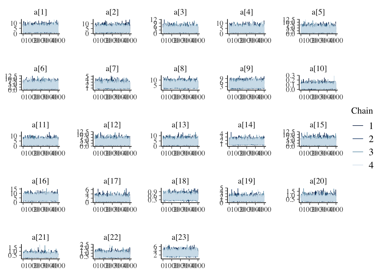

mcmc_trace(draws_b)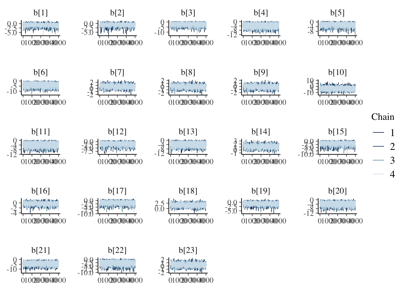

mcmc_trace(draws_theta)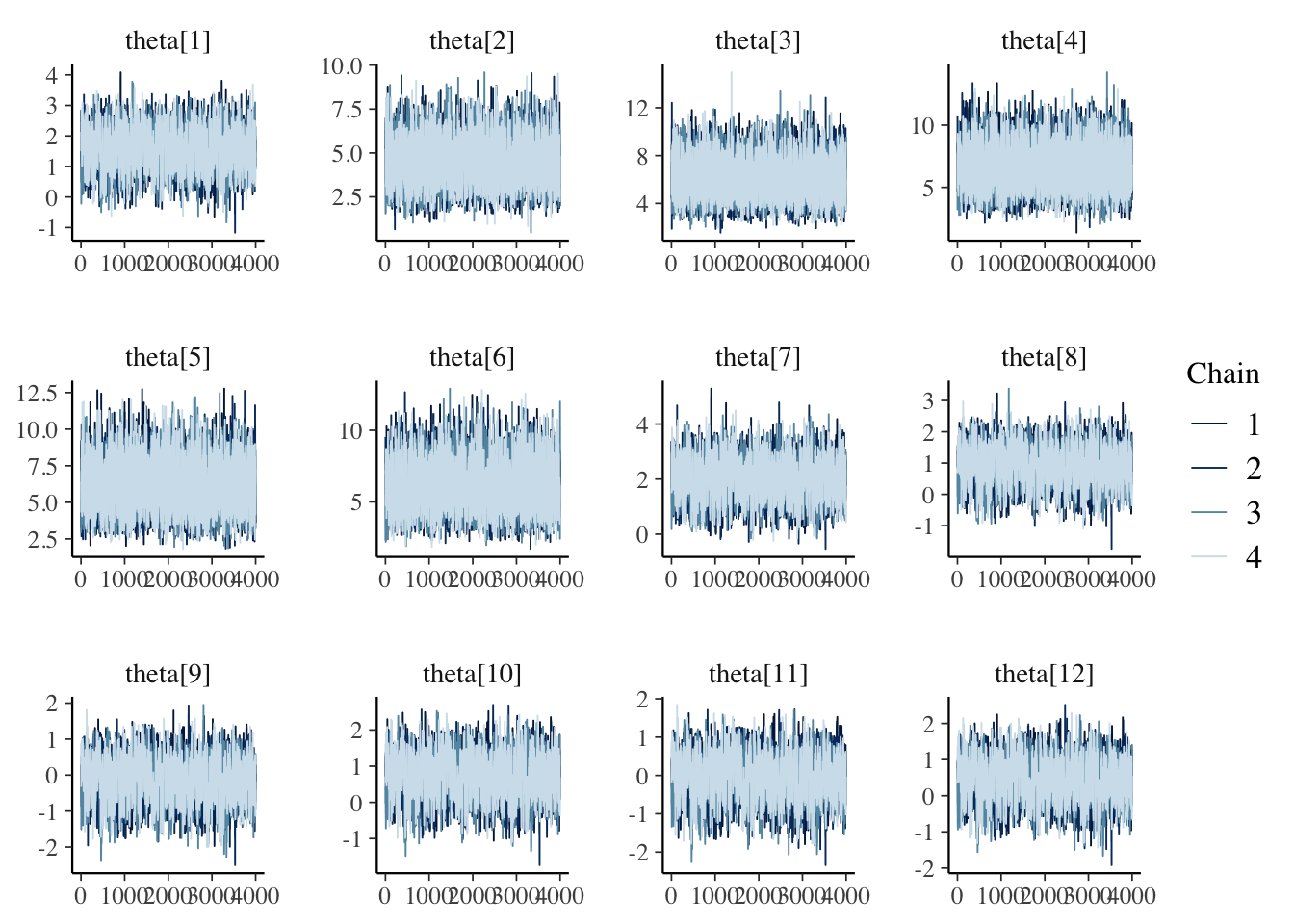

5.3.2 Rhat and Effective samples

fit_pbo$summary(c('a','b', 'theta')) %>% 
  kable(caption='Summary values fit of the model, including effective samples and Rhat', 
      booktabs=T,
      digits =3,
      format='html') %>% 
  kable_styling() %>% 
  scroll_box()

Table 5.1: Summary values fit of the model, including effective samples and Rhat
variable	mean	median	sd	mad	q5	q95	rhat	ess_bulk	ess_tail
a[1]	3.934	3.707	1.837	1.837	1.355	7.305	1.000	10482.518	6617.247
a[2]	3.937	3.701	1.817	1.798	1.391	7.285	1.000	11107.081	6472.795
a[3]	2.713	2.411	1.483	1.351	0.885	5.567	1.000	12066.342	9175.795
a[4]	3.464	3.189	1.716	1.665	1.192	6.686	1.000	21378.536	10784.405
a[5]	2.706	2.367	1.511	1.370	0.888	5.625	1.000	10187.985	8808.061
a[6]	3.460	3.155	1.728	1.671	1.196	6.756	1.000	22233.362	11142.743
a[7]	1.777	1.699	0.565	0.532	1.006	2.816	1.000	9235.783	11044.112
a[8]	5.405	5.220	1.727	1.693	2.877	8.540	1.000	12518.009	11842.410
a[9]	4.112	3.928	1.424	1.379	2.097	6.707	1.000	11774.405	10021.930
a[10]	0.062	0.059	0.031	0.029	0.015	0.117	1.000	6929.124	3558.016
a[11]	3.449	3.170	1.692	1.636	1.206	6.663	1.000	20504.043	11361.605
a[12]	2.916	2.611	1.593	1.532	0.900	5.968	1.000	10505.108	7419.611
a[13]	3.449	3.151	1.722	1.662	1.202	6.678	1.000	21554.343	11428.768
a[14]	1.467	1.408	0.419	0.389	0.890	2.249	1.000	9334.328	10855.270
a[15]	2.943	2.645	1.606	1.527	0.912	6.013	1.000	10472.136	7012.017
a[16]	4.981	4.789	2.025	2.068	2.009	8.585	1.000	13988.593	8593.783
a[17]	1.398	1.274	0.661	0.600	0.571	2.647	1.000	10909.801	8282.476
a[18]	0.497	0.484	0.132	0.126	0.306	0.735	1.001	8682.765	9710.728
a[19]	1.138	1.055	0.470	0.421	0.537	2.014	1.000	8857.538	9008.410
a[20]	0.527	0.491	0.189	0.162	0.289	0.888	1.000	11049.366	11073.602
a[21]	0.428	0.403	0.142	0.125	0.245	0.694	1.001	11939.433	11161.840
a[22]	0.622	0.582	0.231	0.209	0.325	1.056	1.000	10627.937	9775.536
a[23]	2.672	2.581	0.837	0.808	1.467	4.192	1.000	11187.964	9926.076
b[1]	-0.683	-0.629	0.739	0.669	-1.930	0.389	1.002	1619.587	3916.449
b[2]	-0.674	-0.616	0.742	0.672	-1.901	0.397	1.002	1711.981	3375.299
b[3]	-1.988	-1.733	1.347	1.120	-4.570	-0.285	1.001	4367.543	6005.187
b[4]	-3.430	-3.185	1.747	1.710	-6.657	-1.031	1.001	8847.775	10212.229
b[5]	-2.004	-1.759	1.347	1.138	-4.580	-0.277	1.001	4252.917	6468.271
b[6]	-3.469	-3.217	1.771	1.698	-6.777	-1.026	1.000	8131.056	10593.452
b[7]	0.634	0.633	0.581	0.589	-0.326	1.573	1.003	1371.617	2689.014
b[8]	-0.047	-0.041	0.573	0.588	-0.988	0.885	1.003	1285.212	2596.902
b[9]	-0.157	-0.151	0.586	0.598	-1.131	0.795	1.003	1325.181	2864.499
b[10]	-3.540	-3.523	2.295	2.220	-7.331	0.158	1.000	13997.424	8994.802
b[11]	-3.435	-3.179	1.759	1.698	-6.716	-1.038	1.000	9022.686	10282.626
b[12]	-1.500	-1.300	1.158	0.948	-3.673	-0.027	1.001	3084.613	4728.449
b[13]	-3.470	-3.233	1.769	1.729	-6.731	-1.010	1.000	7954.683	9611.534
b[14]	1.101	1.099	0.593	0.608	0.127	2.067	1.003	1465.963	3178.756
b[15]	-1.486	-1.288	1.154	0.928	-3.671	-0.038	1.001	3176.183	4225.810
b[16]	-0.346	-0.331	0.604	0.606	-1.345	0.608	1.002	1349.709	3100.828
b[17]	-1.455	-1.308	1.087	0.957	-3.455	0.009	1.001	3207.599	5478.346
b[18]	1.573	1.578	0.709	0.702	0.401	2.738	1.002	2073.487	4520.739
b[19]	-0.768	-0.695	0.835	0.786	-2.238	0.472	1.002	2082.773	4329.199
b[20]	-3.476	-3.298	1.558	1.481	-6.347	-1.254	1.001	6173.014	8820.348
b[21]	-4.062	-3.890	1.653	1.598	-7.018	-1.678	1.001	6832.772	9577.002
b[22]	-2.553	-2.388	1.367	1.277	-5.032	-0.633	1.001	4999.038	6668.300
b[23]	0.355	0.360	0.571	0.584	-0.595	1.275	1.003	1314.129	2899.819
theta[1]	1.504	1.496	0.633	0.638	0.464	2.545	1.003	1619.499	3267.244
theta[2]	4.385	4.290	1.187	1.150	2.589	6.494	1.001	5924.706	9161.527
theta[3]	6.048	5.931	1.520	1.503	3.761	8.694	1.000	9604.680	9284.926
theta[4]	6.544	6.432	1.614	1.605	4.080	9.362	1.000	11620.501	10261.762
theta[5]	6.041	5.913	1.526	1.483	3.736	8.721	1.001	9097.508	10472.750
theta[6]	6.060	5.944	1.535	1.500	3.725	8.758	1.000	8938.844	9589.486
theta[7]	1.947	1.939	0.675	0.669	0.847	3.077	1.003	1801.573	3782.787
theta[8]	0.885	0.886	0.587	0.601	-0.083	1.850	1.003	1391.774	3299.372
theta[9]	-0.161	-0.155	0.581	0.601	-1.120	0.777	1.003	1303.435	2552.924
theta[10]	0.681	0.679	0.580	0.598	-0.277	1.625	1.003	1363.143	2642.354
theta[11]	-0.084	-0.081	0.565	0.583	-1.021	0.833	1.003	1252.784	2728.216
theta[12]	0.416	0.420	0.567	0.580	-0.518	1.337	1.003	1287.660	2742.103

5.4 Results

fit_summary_a_b <- fit_pbo$summary(c('a','b'))
fit_summary_a <- fit_pbo$summary(c('a'))
fit_summary_b <- fit_pbo$summary(c('b'))
fit_summary_theta <- fit_pbo$summary(c('theta'))

5.4.1 Difficulty and discrimination

Table for the benchmark functions

table_benchmarks <- fit_summary_a_b %>% 
  select('Benchmark ID'=variable, 
         Median=median,
         'CI 5%'=q5,
         'CI 95%'=q95)

table_benchmarks$'Benchmark ID'<-rep(benchmarks,2)

kable(table_benchmarks,
      caption='Summary values of the discrimination and difficulty level parameters for the PBO benchmarks', 
      booktabs=T,
      digits =3,
      format='html',
      linesep = "") %>% 
  kable_styling() %>% 
  pack_rows("Discrimination value (a)",1,23) %>% 
  pack_rows("Difficulty level (b)",23,46)

Table 5.2: Summary values of the discrimination and difficulty level parameters for the PBO benchmarks
Benchmark ID	Median	CI 5%	CI 95%
Discrimination value (a)
1	3.707	1.355	7.305
2	3.701	1.391	7.285
3	2.411	0.885	5.567
4	3.189	1.192	6.686
5	2.367	0.888	5.625
6	3.155	1.196	6.756
7	1.699	1.006	2.816
8	5.220	2.877	8.540
9	3.928	2.097	6.707
10	0.059	0.015	0.117
11	3.170	1.206	6.663
12	2.611	0.900	5.968
13	3.151	1.202	6.678
14	1.408	0.890	2.249
15	2.645	0.912	6.013
16	4.789	2.009	8.585
17	1.274	0.571	2.647
18	0.484	0.306	0.735
19	1.055	0.537	2.014
20	0.491	0.289	0.888
21	0.403	0.245	0.694
22	0.582	0.325	1.056
Difficulty level (b)
23	2.581	1.467	4.192
1	-0.629	-1.930	0.389
2	-0.616	-1.901	0.397
3	-1.733	-4.570	-0.285
4	-3.185	-6.657	-1.031
5	-1.759	-4.580	-0.277
6	-3.217	-6.777	-1.026
7	0.633	-0.326	1.573
8	-0.041	-0.988	0.885
9	-0.151	-1.131	0.795
10	-3.523	-7.331	0.158
11	-3.179	-6.716	-1.038
12	-1.300	-3.673	-0.027
13	-3.233	-6.731	-1.010
14	1.099	0.127	2.067
15	-1.288	-3.671	-0.038
16	-0.331	-1.345	0.608
17	-1.308	-3.455	0.009
18	1.578	0.401	2.738
19	-0.695	-2.238	0.472
20	-3.298	-6.347	-1.254
21	-3.890	-7.018	-1.678
22	-2.388	-5.032	-0.633
23	0.360	-0.595	1.275

mcmc_intervals(draws_a) +
  scale_y_discrete(labels=benchmarks)+
  labs(x='Discrimination parameter (a)',
       y='Benchmark function ID',
       title='Discrimination parameter distribution (PBO)')

## Scale for 'y' is already present. Adding another scale for 'y', which will
## replace the existing scale.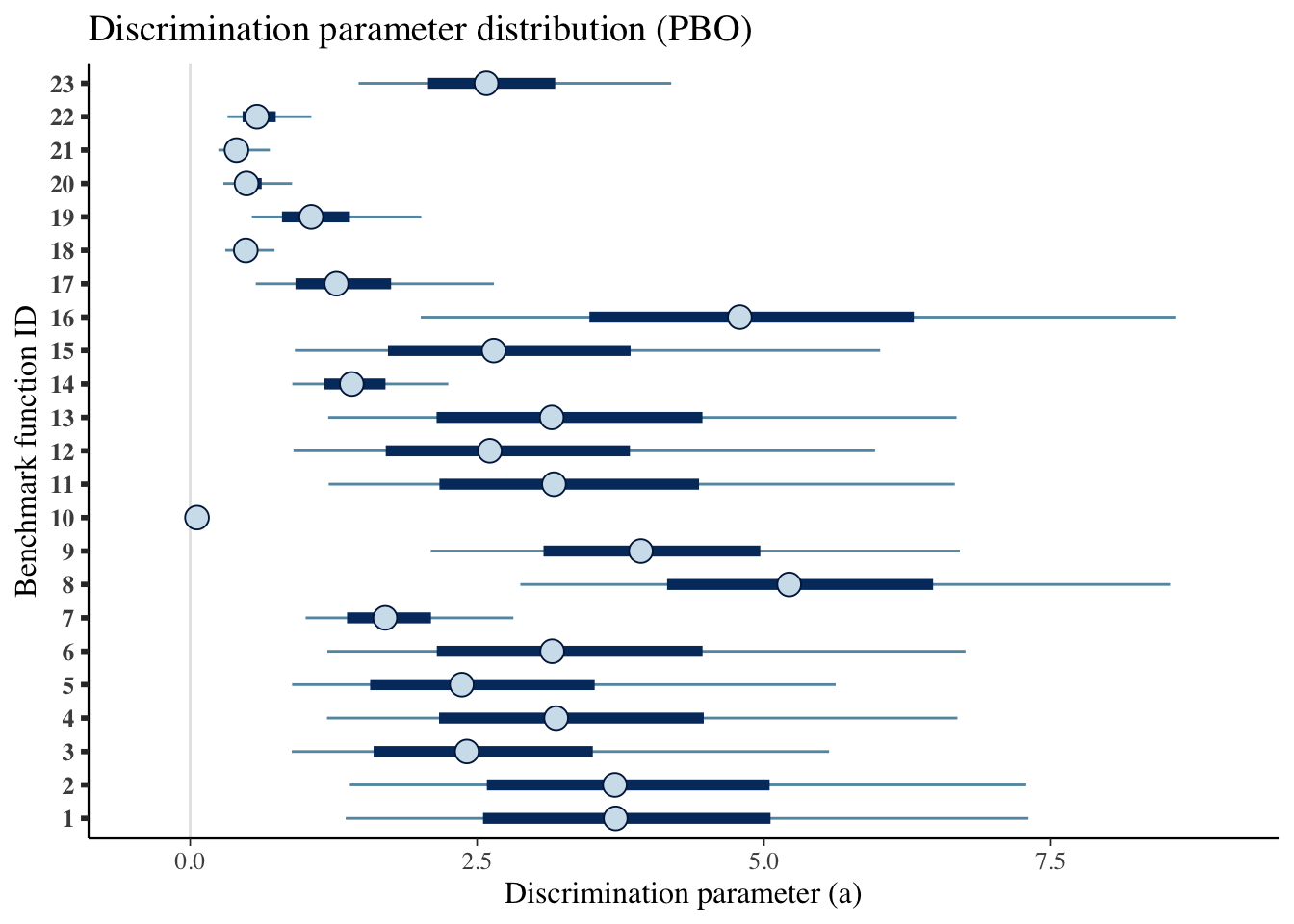

mcmc_intervals(draws_b) +
  scale_y_discrete(labels=benchmarks)+
  labs(x='Difficulty level parameter (b)',
       y='Benchmark function ID',
       title='Difficulty level parameter distribution (PBO)')

## Scale for 'y' is already present. Adding another scale for 'y', which will
## replace the existing scale.

5.4.2 Ability

Creating a table

table_algorithms <- fit_summary_theta %>% 
  select(Algorithms=variable, 
         Median=median,
         'CI 5%'=q5,
         'CI 95%'=q95)

table_algorithms$Algorithms <- algorithms

kable(table_algorithms,
      caption='Summary values of the ability level of the algorithms (PBO)', 
      booktabs=T,
      digits =3,
      format='html',
      linesep = "") %>% 
  kable_styling()

Table 5.3: Summary values of the ability level of the algorithms (PBO)
Algorithms	Median	CI 5%	CI 95%
(1+(λ,λ)) GA	1.496	0.464	2.545
(1+1) EA_>0	4.290	2.589	6.494
(1+1) fGA	5.931	3.761	8.694
(1+10) EA_{r/2,2r}	6.432	4.080	9.362
(1+10) EA_>0	5.913	3.736	8.721
(1+10) EA_logNormal	5.944	3.725	8.758
(1+10) EA_normalized	1.939	0.847	3.077
(1+10) EA_var_ctrl	0.886	-0.083	1.850
(30,30) vGA	-0.155	-1.120	0.777
EDA	0.679	-0.277	1.625
gHC	-0.081	-1.021	0.833
RLS	0.420	-0.518	1.337

mcmc_intervals(draws_theta) +
  scale_y_discrete(labels=algorithms)+
  labs(x=unname(TeX("Ability level ($\\theta$)")),
       y='Algorithm',
       title='Ability level parameter distribution (PBO)')

## Scale for 'y' is already present. Adding another scale for 'y', which will
## replace the existing scale.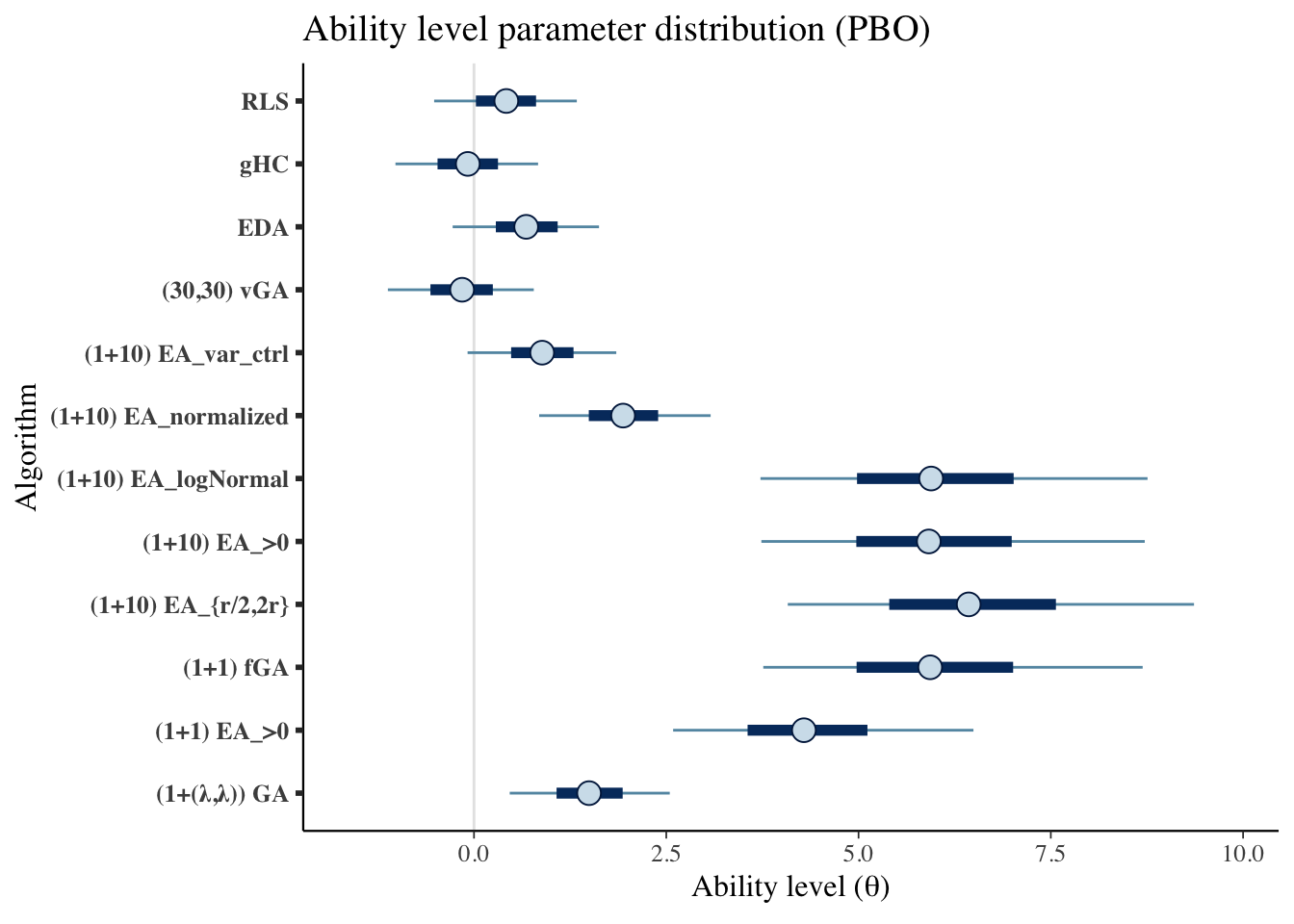

5.4.3 Item information

We will use the same functions from the BBOB case study

Creating a single data frame

item_information_df <- NULL
for(i in seq(1:length(benchmarks))){
  a<-as.matrix(fit_summary_a[i,c(3,6,7)])
  b<-as.matrix(fit_summary_b[i,c(3,6,7)])
  iinfo <- item_info_with_intervals(a=a,b=b,item = i,thetamin = -7, thetamax = 5)
  item_information_df <- rbind(item_information_df,iinfo)
}

Now we can create an information plot for every item

item_information_df %>% 
  pivot_wider(names_from = 'pars', values_from = 'Information') %>% 
  ggplot(aes(x=theta))+
    geom_line(aes(y=median), color='black')+
    # geom_line(aes(y=q05), color='red', linetype='dashed')+
    # geom_line(aes(y=q95), color='blue', linetype='dashed')+
    facet_wrap(~item,
               ncol=4) +
    labs(title='Item information curve (PBO)',
         x=unname(TeX("Ability ($\\theta$)")),
         y='Information',
         color='Information interval')+
    theme_bw() +
    theme(legend.position = 'bottom')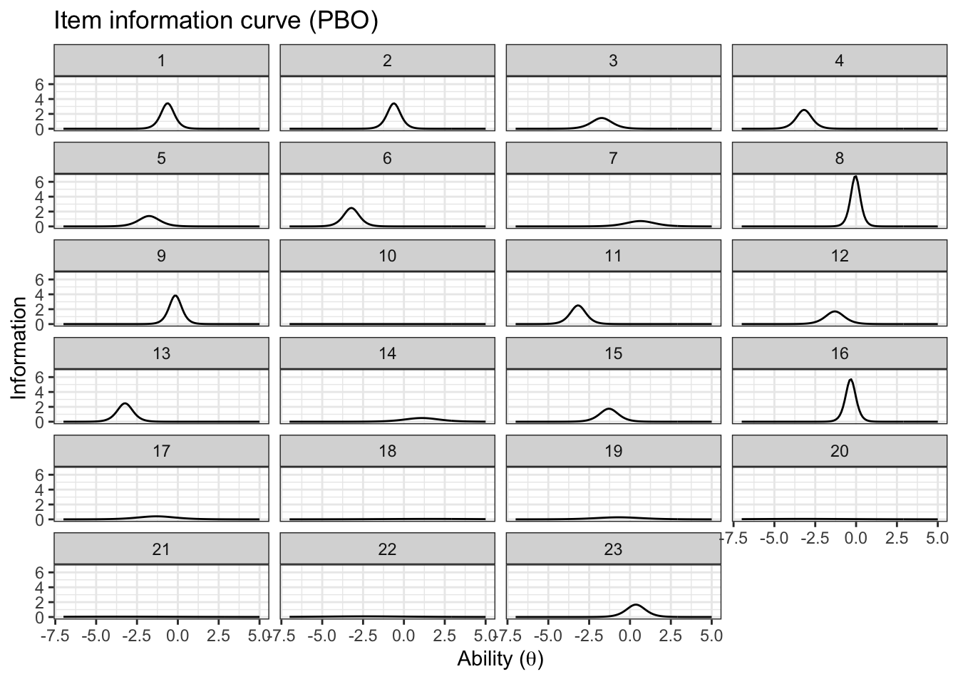

5.4.4 Test information

We can also look at the test information. First, we need to pivot wider so we can sum the items

test_information_df <- item_information_df %>% 
  pivot_wider(names_from = 'item', values_from = 'Information') %>% 
  mutate(TestInfo = dplyr::select(., -theta, -pars) %>% rowSums()) %>% 
  dplyr::select(theta, pars, TestInfo)

Now that we have calculated the test parameters we can plot the test information

First let’s get a horizontal line to show where the algorithms median ability lies

alg_median <- fit_summary_theta %>% 
  mutate(Algorithm=algorithms) %>% 
  select(Algorithm, median)

test_information_df %>% 
  dplyr::select(theta, pars, TestInfo) %>% 
  pivot_wider(names_from = 'pars', values_from = 'TestInfo') %>% 
  ggplot(aes(x=theta)) +
  geom_line(aes(y=median))+
  geom_vline(data=alg_median, aes(xintercept=median,color=Algorithm),linetype='dashed')+
  labs(
    title='Test Information Curve (PBO)',
    x=unname(TeX("Ability ($\\theta$)")),
    y='Test information',
    color='Algorithm median'
  )+
  theme_bw()+
  guides(color=guide_legend(nrow=5,byrow=TRUE))+
  theme(legend.position = 'bottom')