Chapter 6 Extra I: BBOB 2009 and 2019 | Online appendix for the paper: “On the Assessment of Benchmark Suites for Algorithm Comparison”

6.1 Importing the data

To illustrate and make the analysis we will use 5 as the number of dimensions for the benchmark functions

d_bbob2009 <- read_csv('data/bbob2009.csv') %>% 
  select(algId, DIM, funcId, runs, succ, budget) %>% 
  filter(DIM==5)

d_bbob2019 <- read_csv('data/bbob2019.csv') %>% 
  select(algId, DIM, funcId, runs, succ, budget) %>% 
  filter(DIM==5)

d_bbob <- rbind(d_bbob2009, d_bbob2019) %>% 
  mutate(algId_index = as.integer(as.factor(algId)))

#vector with the names in order
benchmarks <- seq(1,24)
algorithms <- levels(as.factor(d_bbob$algId))

6.2 Preparing the Stan data

bbob_standata <- list(
  N = nrow(d_bbob),
  y_succ = as.integer(d_bbob$succ),
  N_tries = as.integer(d_bbob$runs),
  p = d_bbob$algId_index,
  Np = as.integer(length(unique(d_bbob$algId_index))),
  item = as.integer(d_bbob$funcId),
  Nitem = as.integer(length(unique(d_bbob$funcId)))
)

irt2pl <- cmdstan_model('models/irt2pl.stan') 
fit_bbob <- irt2pl$sample(
  data= bbob_standata,
  seed = seed,
  chains = 4,
  iter_sampling = 4000,
  parallel_chains = 4,
  max_treedepth = 15
)
fit_bbob$save_object(file='fitted/bbob-2009-2019-5.RDS')

To load the fitted model to save time in compiling this document

fit_bbob<-readRDS('fitted/bbob-2009-2019-5.RDS')

6.3 Diagnostics

Getting the draws from the posterior

draws_a <- fit_bbob$draws('a')
draws_b <- fit_bbob$draws('b')
draws_theta <- fit_bbob$draws('theta')

6.3.1 Traceplots

mcmc_trace(draws_a)

mcmc_trace(draws_b)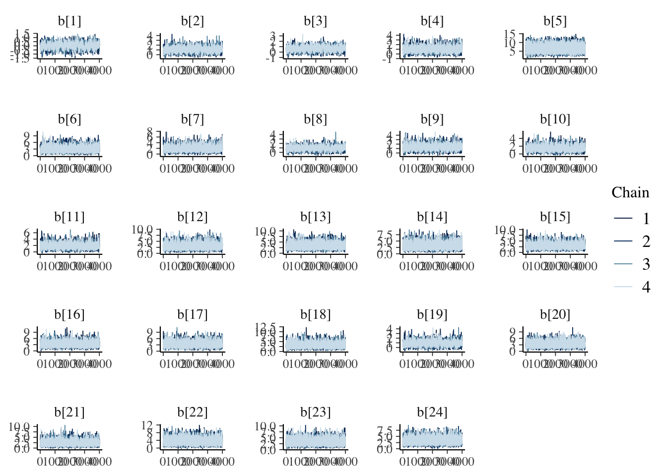

mcmc_trace(draws_theta)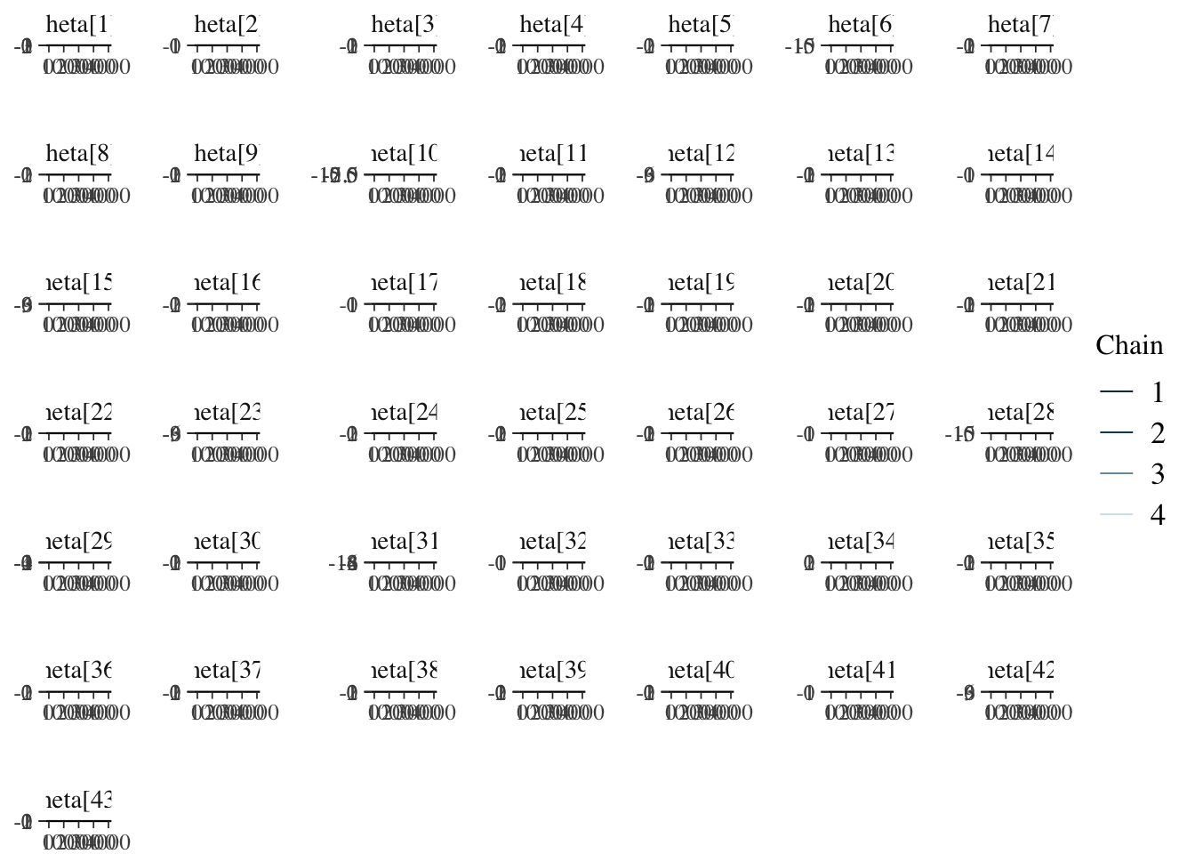

6.4 Results

fit_summary_a_b <- fit_bbob$summary(c('a','b'))
fit_summary_a <- fit_bbob$summary(c('a'))
fit_summary_b <- fit_bbob$summary(c('b'))
fit_summary_theta <- fit_bbob$summary(c('theta'))

6.4.1 Difficulty and discrimination

Table for the benchmark functions

table_benchmarks <- fit_summary_a_b %>% 
  select('Benchmark ID'=variable, 
         Median=median,
         'CI 5%'=q5,
         'CI 95%'=q95)

table_benchmarks$'Benchmark ID'<-rep(benchmarks,2)

kable(table_benchmarks,
      caption='Summary values of the discrimination and difficulty level parameters for the BBOB-2009 benchmarks', 
      booktabs=T,
      digits =3,
      format='html',
      linesep = "") %>% 
  kable_styling() %>% 
  pack_rows("Discrimination value (a)",1,24) %>% 
  pack_rows("Difficulty level (b)",25,48)

Table 6.1: Summary values of the discrimination and difficulty level parameters for the BBOB-2009 benchmarks
Benchmark ID	Median	CI 5%	CI 95%
Discrimination value (a)
1	5.316	3.835	7.369
2	1.887	1.201	2.779
3	2.132	1.365	3.182
4	1.446	0.823	2.379
5	0.053	0.033	0.085
6	0.877	0.497	1.483
7	1.117	0.608	1.932
8	2.068	1.344	2.998
9	1.624	0.996	2.463
10	1.541	0.907	2.360
11	1.326	0.755	2.096
12	0.877	0.505	1.480
13	0.801	0.461	1.361
14	0.801	0.464	1.367
15	0.789	0.457	1.310
16	0.805	0.467	1.357
17	0.800	0.472	1.366
18	0.801	0.466	1.364
19	1.786	1.043	2.794
20	0.730	0.436	1.216
21	0.823	0.436	1.529
22	0.476	0.270	1.015
23	0.800	0.469	1.363
24	0.804	0.467	1.359
Difficulty level (b)
1	0.009	-0.621	0.624
2	0.976	0.217	1.865
3	0.569	-0.131	1.302
4	0.858	0.062	1.857
5	6.603	3.765	10.043
6	2.657	1.281	5.048
7	1.666	0.620	3.413
8	0.856	0.134	1.665
9	1.206	0.382	2.234
10	1.293	0.455	2.485
11	1.603	0.649	3.122
12	2.706	1.319	4.982
13	3.032	1.511	5.580
14	2.960	1.447	5.415
15	2.618	1.270	4.863
16	3.013	1.514	5.479
17	3.045	1.509	5.448
18	2.990	1.481	5.465
19	0.805	0.057	1.723
20	3.018	1.525	5.389
21	2.130	0.796	4.427
22	3.423	1.250	6.472
23	3.029	1.502	5.482
24	2.976	1.487	5.450

mcmc_intervals(draws_a) +
  scale_y_discrete(labels=benchmarks)+
  labs(x='Discrimination parameter (a)',
       y='Benchmark function ID',
       title='Discrimination parameter distribution (BBOB-2009)')

## Scale for 'y' is already present. Adding another scale for 'y', which will
## replace the existing scale.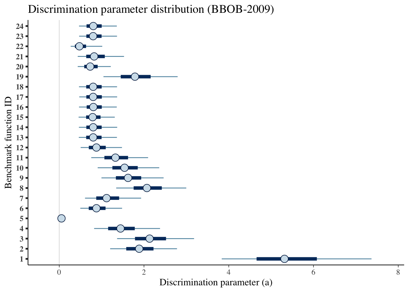

mcmc_intervals(draws_b) +
  scale_y_discrete(labels=benchmarks)+
  labs(x='Difficulty level parameter (b)',
       y='Benchmark function ID',
       title='Difficulty level parameter distribution (BBOB-2009)')

## Scale for 'y' is already present. Adding another scale for 'y', which will
## replace the existing scale.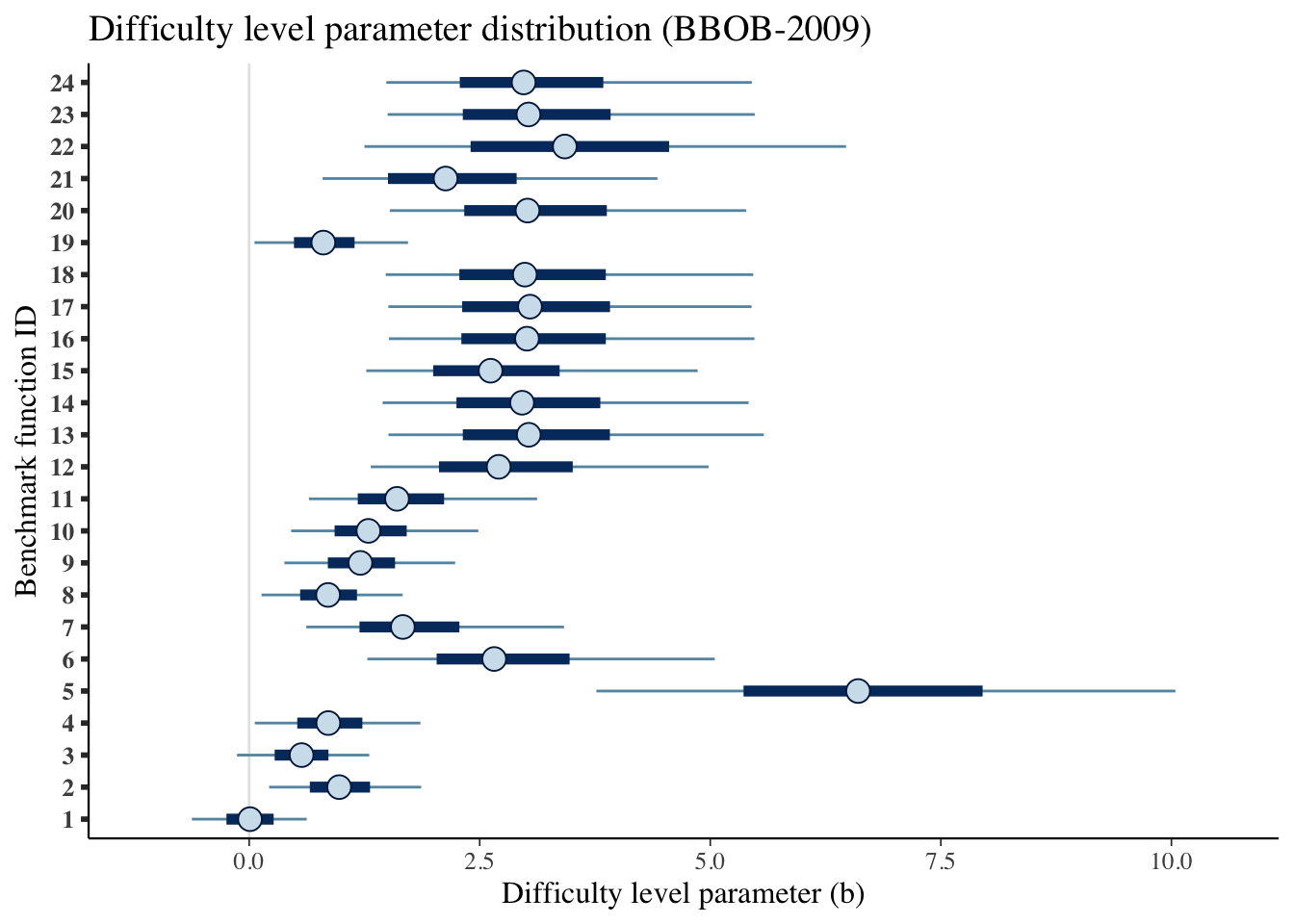

6.4.2 Ability

Creating a table

table_algorithms <- fit_summary_theta %>% 
  select(Algorithms=variable, 
         Median=median,
         'CI 5%'=q5,
         'CI 95%'=q95)

table_algorithms$Algorithms <- algorithms

kable(table_algorithms,
      caption='Summary values of the ability level of the algorithms (BBOB-2009)',
      booktabs=T,
      digits =3,
      format='html',
      linesep = "") %>% 
  kable_styling()

Table 6.2: Summary values of the ability level of the algorithms (BBOB-2009)
Algorithms	Median	CI 5%	CI 95%
adapt-Nelder-Mead-scipy-2019	-0.820	-1.641	-0.085
Adaptive_Two_Mode	-0.147	-0.797	0.500
ALPS	-0.569	-1.242	0.081
AMALGAM	-0.540	-1.215	0.110
BAYEDA	-0.570	-1.253	0.085
BFGS	-5.993	-9.393	-3.547
BFGS-scipy-2019	-0.442	-1.103	0.204
BIPOP-CMA-ES	-0.567	-1.257	0.086
Cauchy-EDA	-0.561	-1.234	0.095
CG-scipy-2019	-4.277	-6.687	-2.495
CMA-ESPLUSSEL	-0.568	-1.251	0.089
COBYLA-scipy-2019	-4.279	-6.793	-2.518
DASA	-0.570	-1.246	0.086
DE-PSO	-0.331	-0.981	0.298
DE-scipy-2019	-4.263	-6.758	-2.506
EDA-PSO	-0.542	-1.223	0.098
FULLNEWUOA	0.104	-0.529	0.723
G3PCX	-0.540	-1.224	0.109
GA	-0.570	-1.239	0.087
GLOBAL	-0.569	-1.246	0.084
iAMALGAM	-0.335	-0.991	0.301
IPOP-SEP-CMA-ES	-0.514	-1.193	0.129
L-BFGS-B-scipy-2019	-4.272	-6.810	-2.487
LSfminbnd	-0.521	-1.197	0.124
LSstep	-0.428	-1.086	0.215
MA-LS-CHAIN	-0.526	-1.206	0.120
MCS	0.271	-0.365	0.900
NELDER	-5.998	-9.444	-3.478
Nelder-Mead-scipy-2019	-1.591	-2.718	-0.663
NELDERDOERR	-0.472	-1.137	0.173
NEWUOA	-5.996	-9.352	-3.501
ONEFIFTH	-0.264	-0.911	0.368
POEMS	-0.527	-1.205	0.123
Powell-scipy-2019	0.718	0.055	1.371
PSO	-0.512	-1.188	0.135
PSO_Bounds	-0.566	-1.247	0.080
RANDOMSEARCH	-0.573	-1.252	0.090
Rosenbrock	-0.549	-1.229	0.101
RS-4-initIn0	-0.567	-1.251	0.080
RS-5-initIn0	-0.572	-1.242	0.084
RS-6-initIn0	-0.255	-0.902	0.375
TNC-scipy-2019	-4.275	-6.695	-2.522
VNS	-0.563	-1.247	0.078

mcmc_intervals(draws_theta) +
  scale_y_discrete(labels=algorithms)+
  labs(x=unname(TeX("Ability level ($\\theta$)")),
       y='Algorithm',
       title='Ability level parameter distribution (BBOB-2009)')

## Scale for 'y' is already present. Adding another scale for 'y', which will
## replace the existing scale.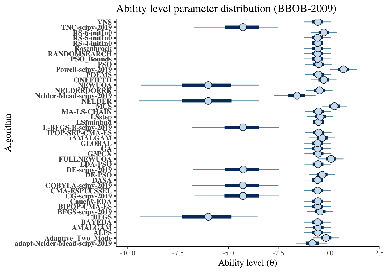

6.4.3 Item information

Now we can create an information plot for every item

item_information_df <- NULL
for(i in seq(1:length(benchmarks))){
  a<-as.matrix(fit_summary_a[i,c(3,6,7)])
  b<-as.matrix(fit_summary_b[i,c(3,6,7)])
  iinfo <- item_info_with_intervals(a=a,b=b,item = i,thetamin = -7, thetamax = 5)
  item_information_df <- rbind(item_information_df,iinfo)
}

Now we can create an information plot for every item

item_information_df %>% 
  pivot_wider(names_from = 'pars', values_from = 'Information') %>% 
  ggplot(aes(x=theta))+
    geom_line(aes(y=median), color='black')+
    # geom_line(aes(y=q05), color='red', linetype='dashed')+
    # geom_line(aes(y=q95), color='blue', linetype='dashed')+
    facet_wrap(~item,
               ncol=4) +
    labs(title='Item information curve (BBOB-2009)',
         x=unname(TeX("Ability ($\\theta$)")),
         y='Information',
         color='Information interval')+
    theme_bw() +
    theme(legend.position = 'bottom')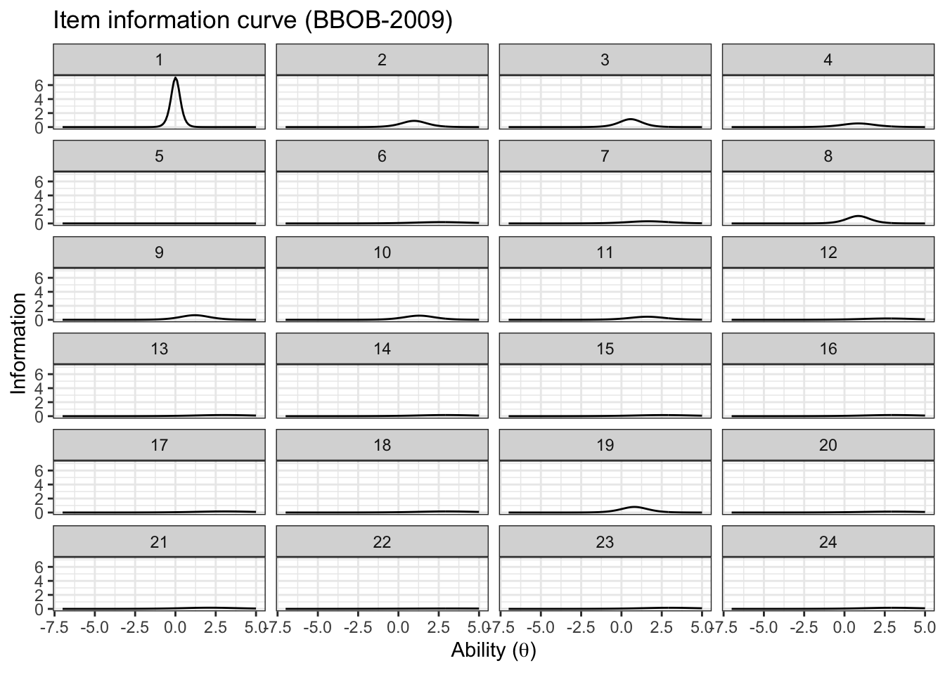

6.4.4 Test information

We can also look at the test information. First, we need to pivot wider so we can sum the items

test_information_df <- item_information_df %>% 
  pivot_wider(names_from = 'item', values_from = 'Information') %>% 
  mutate(TestInfo = dplyr::select(., -theta, -pars) %>% rowSums()) %>% 
  dplyr::select(theta, pars, TestInfo)

Now that we have calculated the test parameters we can plot the test information

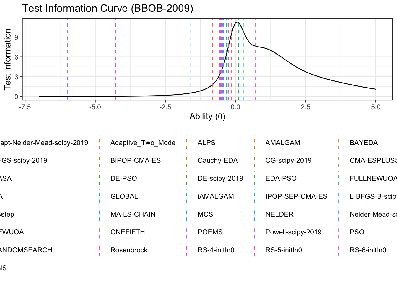
First let’s get a horizontal line to show where the algorithms median ability lies

alg_median <- fit_summary_theta %>% 
  mutate(Algorithm=algorithms) %>% 
  select(Algorithm, median)

test_information_df %>% 
  dplyr::select(theta, pars, TestInfo) %>% 
  pivot_wider(names_from = 'pars', values_from = 'TestInfo') %>% 
  ggplot(aes(x=theta)) +
  geom_line(aes(y=median))+
  geom_vline(data=alg_median, aes(xintercept=median,color=Algorithm),linetype='dashed')+
  labs(
    title='Test Information Curve (BBOB-2009)',
    x=unname(TeX("Ability ($\\theta$)")),
    y='Test information',
    color='Algorithm median'
  )+
  theme_bw()+
  guides(color=guide_legend(nrow=8,byrow=TRUE))+
  theme(legend.position = 'bottom')