Chapter 4 Case Study I: BBOB 2019 | Online appendix for the paper: “On the Assessment of Benchmark Suites for Algorithm Comparison”

4.1 Importing the data

To illustrate and make the analysis, we will the number of dimensions equal to 5 (since the benchmark functions are all scalable). To do an analysis with different dimensions just change the code here

d_bbob <- read_csv('data/bbob2019.csv') %>% 
  select(algId, DIM, funcId, runs, succ, budget) %>% 
  filter(DIM==5) %>%  
  mutate(algId_index = as.integer(as.factor(algId)))

#vector with the names in order
benchmarks <- seq(1,24)
algorithms <- levels(as.factor(d_bbob$algId))

4.2 Preparing the Stan data

Creating a list for Stan.

bbob_standata <- list(
  N = nrow(d_bbob),
  y_succ = as.integer(d_bbob$succ),
  N_tries = as.integer(d_bbob$runs),
  p = d_bbob$algId_index,
  Np = as.integer(length(unique(d_bbob$algId_index))),
  item = as.integer(d_bbob$funcId),
  Nitem = as.integer(length(unique(d_bbob$funcId)))
)

Calling the model with cmdstanr

irt2pl <- cmdstan_model('models/irt2pl.stan') 
fit_bbob <- irt2pl$sample(
  data= bbob_standata,
  chains = 4,
  iter_sampling = 4000,
  parallel_chains = 4,
  max_treedepth = 15
)
fit_bbob$save_object(file='fitted/bbob5.RDS')

To load the fitted model (to save time in compiling this document)

fit_bbob<-readRDS('fitted/bbob5.RDS')

4.3 Diagnostics

Getting the draws from the posterior

draws_a <- fit_bbob$draws('a')
draws_b <- fit_bbob$draws('b')
draws_theta <- fit_bbob$draws('theta')

4.3.1 Traceplots

mcmc_trace(draws_a)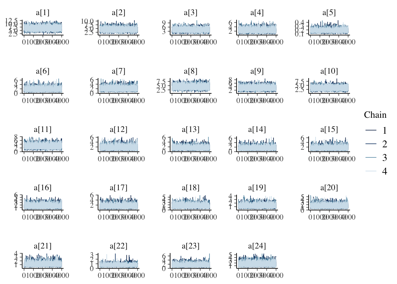

mcmc_trace(draws_b)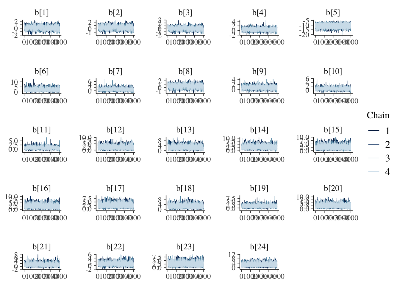

mcmc_trace(draws_theta)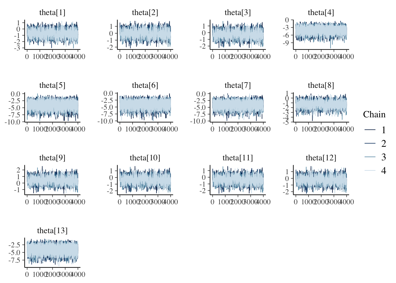

4.3.2 Rhat and Effective samples

fit_bbob$summary(c('a','b', 'theta')) %>% 
  kable(caption='Summary values fit of the model, including effective samples and Rhat', 
      booktabs=T,
      digits =3,
      format='html') %>% 
  kable_styling() %>% 
  scroll_box()

Table 4.1: Summary values fit of the model, including effective samples and Rhat
variable	mean	median	sd	mad	q5	q95	rhat	ess_bulk	ess_tail
a[1]	6.522	6.430	1.424	1.420	4.318	9.009	1.000	14280.165	11093.421
a[2]	4.324	4.250	1.138	1.115	2.598	6.321	1.000	12287.535	9783.007
a[3]	4.020	3.931	1.189	1.173	2.216	6.127	1.000	10109.111	9225.800
a[4]	2.414	2.328	0.859	0.852	1.181	3.964	1.000	9537.022	8863.253
a[5]	0.184	0.179	0.040	0.038	0.127	0.255	1.001	9960.494	11299.490
a[6]	1.692	1.565	0.762	0.714	0.691	3.139	1.000	9466.497	6907.590
a[7]	1.939	1.821	0.789	0.742	0.865	3.392	1.000	8753.252	6591.984
a[8]	4.318	4.244	1.128	1.095	2.607	6.312	1.000	12418.532	10295.961
a[9]	3.290	3.213	1.042	1.031	1.714	5.119	1.000	11748.731	8343.076
a[10]	3.266	3.192	1.056	1.042	1.665	5.118	1.000	9944.351	6922.556
a[11]	2.939	2.848	1.015	0.996	1.424	4.730	1.001	10865.103	7069.033
a[12]	1.685	1.554	0.764	0.726	0.693	3.123	1.000	9145.424	7175.492
a[13]	1.478	1.347	0.670	0.612	0.629	2.763	1.000	10919.706	8940.304
a[14]	1.478	1.343	0.676	0.606	0.641	2.775	1.001	11612.301	9517.923
a[15]	1.473	1.355	0.666	0.613	0.634	2.707	1.000	9236.735	7824.179
a[16]	1.482	1.347	0.670	0.608	0.641	2.758	1.000	9694.299	7818.154
a[17]	1.476	1.345	0.674	0.618	0.628	2.734	1.001	9164.008	8435.066
a[18]	1.484	1.356	0.666	0.609	0.640	2.761	1.000	10599.824	8511.088
a[19]	1.182	1.113	0.457	0.412	0.576	2.044	1.000	11309.124	8818.726
a[20]	1.388	1.275	0.624	0.582	0.598	2.572	1.000	9183.205	7985.132
a[21]	1.023	0.939	0.439	0.379	0.477	1.857	1.000	8203.122	8222.777
a[22]	0.670	0.632	0.247	0.221	0.347	1.115	1.001	7799.858	8398.404
a[23]	1.495	1.355	0.691	0.631	0.630	2.813	1.000	10373.600	8546.457
a[24]	1.469	1.340	0.675	0.608	0.620	2.766	1.000	10191.232	8757.702
b[1]	0.190	0.189	0.526	0.517	-0.675	1.049	1.003	1655.798	3234.633
b[2]	0.421	0.418	0.537	0.529	-0.458	1.301	1.003	1714.585	3269.607
b[3]	0.126	0.120	0.532	0.528	-0.750	0.999	1.003	1662.807	3212.317
b[4]	0.400	0.384	0.582	0.572	-0.532	1.366	1.003	1815.237	3702.849
b[5]	-10.606	-10.553	1.755	1.745	-13.618	-7.825	1.000	9271.595	11117.350
b[6]	1.987	1.784	1.170	0.969	0.476	4.159	1.001	4259.516	6617.055
b[7]	0.788	0.734	0.711	0.633	-0.260	1.992	1.002	2240.195	4102.527
b[8]	0.421	0.420	0.536	0.526	-0.463	1.306	1.003	1742.331	3435.551
b[9]	0.678	0.657	0.590	0.561	-0.248	1.668	1.002	2018.667	3758.684
b[10]	0.690	0.667	0.600	0.572	-0.247	1.680	1.002	2031.685	3763.513
b[11]	0.824	0.788	0.651	0.591	-0.148	1.884	1.001	2192.201	3938.860
b[12]	1.993	1.802	1.164	0.998	0.492	4.163	1.001	4568.658	6773.007
b[13]	2.420	2.202	1.295	1.138	0.709	4.876	1.000	5568.265	7220.730
b[14]	2.413	2.204	1.276	1.138	0.713	4.800	1.001	5160.159	6932.234
b[15]	2.419	2.182	1.298	1.123	0.747	4.936	1.001	4644.611	7607.595
b[16]	2.400	2.195	1.266	1.129	0.717	4.822	1.001	5039.876	7317.296
b[17]	2.420	2.195	1.290	1.142	0.715	4.873	1.001	5288.295	7216.751
b[18]	2.401	2.191	1.280	1.132	0.719	4.779	1.001	5412.655	7130.342
b[19]	1.432	1.336	0.880	0.793	0.186	2.976	1.001	3445.220	5449.716
b[20]	2.406	2.178	1.298	1.140	0.714	4.874	1.001	5362.057	6661.986
b[21]	1.239	1.138	0.905	0.829	-0.056	2.847	1.001	3242.422	4953.712
b[22]	0.810	0.734	0.830	0.763	-0.397	2.233	1.002	3062.358	4872.259
b[23]	2.398	2.192	1.286	1.155	0.702	4.841	1.001	5267.369	6601.671
b[24]	2.441	2.218	1.307	1.153	0.721	4.945	1.001	5375.168	7470.779
theta[1]	-0.691	-0.690	0.553	0.542	-1.604	0.212	1.003	1792.092	3591.987
theta[2]	-0.024	-0.024	0.528	0.519	-0.892	0.838	1.003	1681.458	3361.608
theta[3]	-0.255	-0.254	0.532	0.523	-1.131	0.624	1.003	1656.443	3263.409
theta[4]	-3.989	-3.911	1.205	1.175	-6.100	-2.172	1.000	7015.079	9333.640
theta[5]	-4.003	-3.904	1.230	1.185	-6.193	-2.156	1.000	7087.536	9941.552
theta[6]	-3.993	-3.896	1.201	1.171	-6.094	-2.180	1.000	7278.511	9311.373
theta[7]	-4.002	-3.912	1.229	1.200	-6.159	-2.152	1.000	7797.899	8536.771
theta[8]	-1.284	-1.271	0.634	0.621	-2.345	-0.284	1.002	2255.589	4664.016
theta[9]	0.436	0.433	0.523	0.519	-0.430	1.292	1.003	1642.108	2997.515
theta[10]	-0.359	-0.356	0.537	0.529	-1.250	0.518	1.003	1664.464	3065.114
theta[11]	-0.359	-0.360	0.538	0.535	-1.243	0.521	1.003	1652.009	3192.851
theta[12]	-0.232	-0.235	0.532	0.524	-1.110	0.644	1.003	1663.252	3203.973
theta[13]	-4.002	-3.899	1.220	1.195	-6.193	-2.180	1.000	7255.309	8999.452

4.4 Results

Let’s get some summary descriptive statistics of the posterior

fit_summary_a_b <- fit_bbob$summary(c('a','b'))
fit_summary_a <- fit_bbob$summary(c('a'))
fit_summary_b <- fit_bbob$summary(c('b'))
fit_summary_theta <- fit_bbob$summary(c('theta'))

4.4.1 Difficulty and discrimination

Table for the benchmark functions

table_benchmarks <- fit_summary_a_b %>% 
  select('Benchmark ID'=variable, 
         Median=median,
         'CI 5%'=q5,
         'CI 95%'=q95)

table_benchmarks$'Benchmark ID'<-rep(benchmarks,2)

kable(table_benchmarks,
      caption='Summary values of the discrimination and difficulty level parameters for the BBOB benchmarks', 
      booktabs=T,
      digits =3,
      format='html',
      linesep = "") %>% 
  kable_styling() %>% 
  pack_rows("Discrimination value (a)",1,24) %>% 
  pack_rows("Difficulty level (b)",25,48)

Table 4.2: Summary values of the discrimination and difficulty level parameters for the BBOB benchmarks
Benchmark ID	Median	CI 5%	CI 95%
Discrimination value (a)
1	6.430	4.318	9.009
2	4.250	2.598	6.321
3	3.931	2.216	6.127
4	2.328	1.181	3.964
5	0.179	0.127	0.255
6	1.565	0.691	3.139
7	1.821	0.865	3.392
8	4.244	2.607	6.312
9	3.213	1.714	5.119
10	3.192	1.665	5.118
11	2.848	1.424	4.730
12	1.554	0.693	3.123
13	1.347	0.629	2.763
14	1.343	0.641	2.775
15	1.355	0.634	2.707
16	1.347	0.641	2.758
17	1.345	0.628	2.734
18	1.356	0.640	2.761
19	1.113	0.576	2.044
20	1.275	0.598	2.572
21	0.939	0.477	1.857
22	0.632	0.347	1.115
23	1.355	0.630	2.813
24	1.340	0.620	2.766
Difficulty level (b)
1	0.189	-0.675	1.049
2	0.418	-0.458	1.301
3	0.120	-0.750	0.999
4	0.384	-0.532	1.366
5	-10.553	-13.618	-7.825
6	1.784	0.476	4.159
7	0.734	-0.260	1.992
8	0.420	-0.463	1.306
9	0.657	-0.248	1.668
10	0.667	-0.247	1.680
11	0.788	-0.148	1.884
12	1.802	0.492	4.163
13	2.202	0.709	4.876
14	2.204	0.713	4.800
15	2.182	0.747	4.936
16	2.195	0.717	4.822
17	2.195	0.715	4.873
18	2.191	0.719	4.779
19	1.336	0.186	2.976
20	2.178	0.714	4.874
21	1.138	-0.056	2.847
22	0.734	-0.397	2.233
23	2.192	0.702	4.841
24	2.218	0.721	4.945

A more visual representation.

mcmc_intervals(draws_a) +
  scale_y_discrete(labels=benchmarks)+
  labs(x='Discrimination parameter (a)',
       y='Benchmark function ID',
       title='Discrimination parameter distribution (BBOB)')

## Scale for 'y' is already present. Adding another scale for 'y', which will
## replace the existing scale.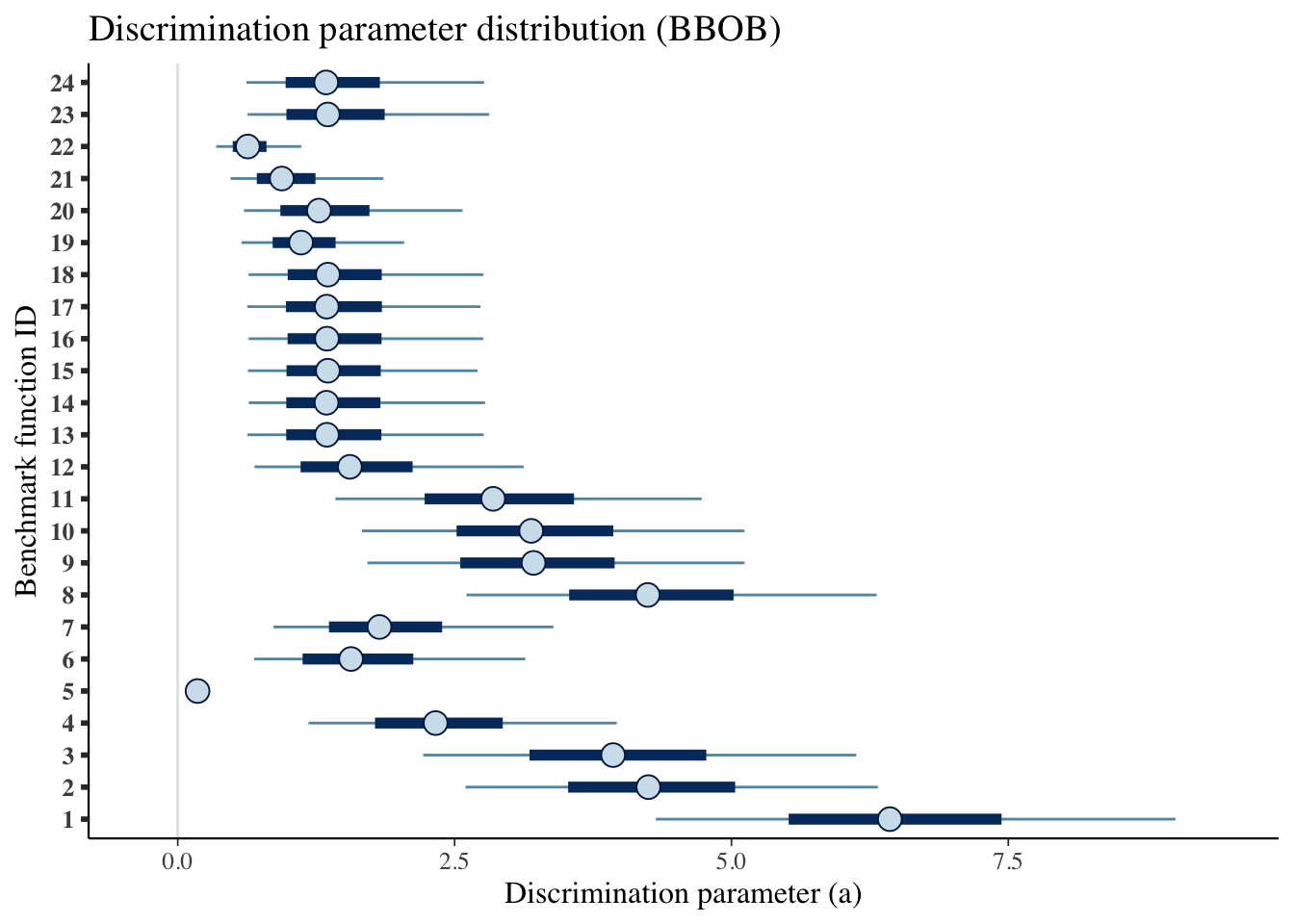

mcmc_intervals(draws_b) +
  scale_y_discrete(labels=benchmarks)+
  labs(x='Difficulty level parameter (b)',
       y='Benchmark function ID',
       title='Difficulty level parameter distribution (BBOB)')

## Scale for 'y' is already present. Adding another scale for 'y', which will
## replace the existing scale.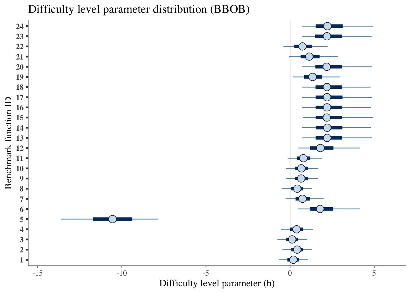

4.4.2 Ability

Creating a table:

table_algorithms <- fit_summary_theta %>% 
  select(Algorithms=variable, 
         Median=median,
         'CI 5%'=q5,
         'CI 95%'=q95)

table_algorithms$Algorithms <- algorithms

kable(table_algorithms,
      caption='Summary values of the ability level of the algorithms (BBOB)',
      booktabs=T,
      digits =3,
      format='html',
      linesep = "") %>% 
  kable_styling()

Table 4.3: Summary values of the ability level of the algorithms (BBOB)
Algorithms	Median	CI 5%	CI 95%
adapt-Nelder-Mead-scipy-2019	-0.690	-1.604	0.212
Adaptive_Two_Mode	-0.024	-0.892	0.838
BFGS-scipy-2019	-0.254	-1.131	0.624
CG-scipy-2019	-3.911	-6.100	-2.172
COBYLA-scipy-2019	-3.904	-6.193	-2.156
DE-scipy-2019	-3.896	-6.094	-2.180
L-BFGS-B-scipy-2019	-3.912	-6.159	-2.152
Nelder-Mead-scipy-2019	-1.271	-2.345	-0.284
Powell-scipy-2019	0.433	-0.430	1.292
RS-4-initIn0	-0.356	-1.250	0.518
RS-5-initIn0	-0.360	-1.243	0.521
RS-6-initIn0	-0.235	-1.110	0.644
TNC-scipy-2019	-3.899	-6.193	-2.180

A more visual representation.

mcmc_intervals(draws_theta) +
  scale_y_discrete(labels=algorithms)+
  labs(x=unname(TeX("Ability level ($\\theta$)")),
       y='Algorithm',
       title='Ability level parameter distribution (BBOB)')

## Scale for 'y' is already present. Adding another scale for 'y', which will
## replace the existing scale.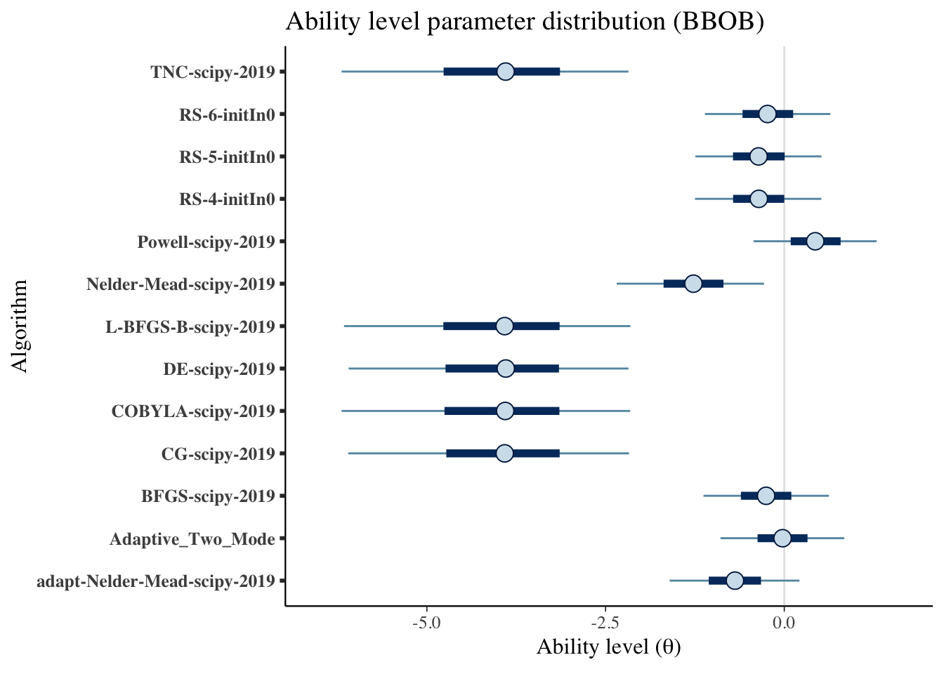

4.4.3 Item information

First let’s create a few helper functions to calculate the item information

p_info <- function(a,b, theta){
     return(exp(a*(theta-b))/(1+exp(a*(theta-b))))
  }
q_info <- function(a,b, theta){
    return(1-p_info(a,b, theta))
  }
#a and b are a vector of 3 a[1] is lower q05 a[2] is median and a[3] is q95
#return a data frame ready to be plottted
item_info_with_intervals <- function(a,b,item, thetamin=-5, thetamax=5,step=0.1){
  theta <- seq(from=thetamin, to=thetamax, by=step)
  info_median <- a[1]^2*p_info(a[1],b[1],theta)*q_info(a[1],b[1],theta)
  info_lower <- a[2]^2*p_info(a[2],b[2],theta)*q_info(a[2],b[2],theta)
  info_higher <- a[3]^2*p_info(a[3],b[3],theta)*q_info(a[3],b[3],theta)
  
  out<- data.frame(Information= c(info_lower,info_median,info_higher),
                   theta=c(theta,theta,theta),
                   pars=c(rep('q05',length(theta)),
                           rep('median',length(theta)),
                           rep('q95',length(theta))),
                   item=c(rep(item,length(theta)),
                          rep(item,length(theta)),
                          rep(item,length(theta))))
  return(out)
}

Creating a single data frame

item_information_df <- NULL
for(i in seq(1:length(benchmarks))){
  a<-as.matrix(fit_summary_a[i,c(3,6,7)])
  b<-as.matrix(fit_summary_b[i,c(3,6,7)])
  iinfo <- item_info_with_intervals(a=a,b=b,item = i,thetamin = -7, thetamax = 5)
  item_information_df <- rbind(item_information_df,iinfo)
}

Now we can create an information plot for every item

item_information_df %>% 
  pivot_wider(names_from = 'pars', values_from = 'Information') %>% 
  ggplot(aes(x=theta))+
    geom_line(aes(y=median), color='black')+
    facet_wrap(~item,
               ncol=4) +
    labs(title='Item information curve (BBOB)',
         x=unname(TeX("Ability ($\\theta$)")),
         y='Information',
         color='Information interval')+
    theme_bw() +
    theme(legend.position = 'bottom')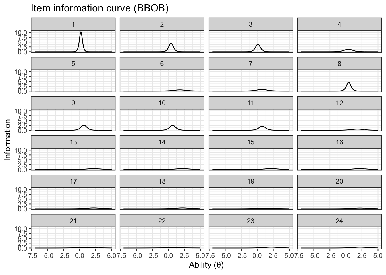

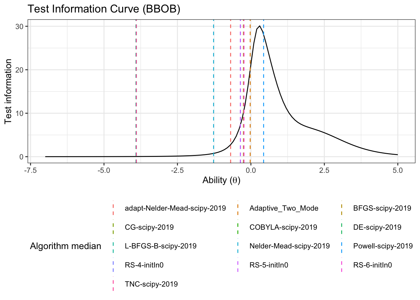
4.4.4 Test information

We can also look at the test information. First, we need to pivot wider so we can sum the items

test_information_df <- item_information_df %>% 
  pivot_wider(names_from = 'item', values_from = 'Information') %>% 
  mutate(TestInfo = dplyr::select(., -theta, -pars) %>% rowSums()) %>% 
  dplyr::select(theta, pars, TestInfo)

Now that we have calculated the test parameters we can plot the test information

First let’s get a horizontal line to show where the algorithms median ability lies

alg_median <- fit_summary_theta %>% 
  mutate(Algorithm=algorithms) %>% 
  select(Algorithm, median)

test_information_df %>% 
  dplyr::select(theta, pars, TestInfo) %>% 
  pivot_wider(names_from = 'pars', values_from = 'TestInfo') %>% 
  ggplot(aes(x=theta)) +
  geom_line(aes(y=median))+
  geom_vline(data=alg_median, aes(xintercept=median,color=Algorithm),linetype='dashed')+
  labs(
    title='Test Information Curve (BBOB)',
    x=unname(TeX("Ability ($\\theta$)")),
    y='Test information',
    color='Algorithm median'
  )+
  theme_bw()+
  guides(color=guide_legend(nrow=5,byrow=TRUE))+
  theme(legend.position = 'bottom')