Chapter 5 Re-analysis 3 | Online appendix for the paper: “Bayesian Paired-Comparison with the bpcs package”

5.1 Importing the data

The data from this paper was made available upon request and below we exemplify a few rows of how the original dataset looks like. Let’s starting importing the data.

d<-read.table("data/MHLC.txt", sep="\t", header=T)
d<-as.data.frame(d)
sample_n(d, size=5) %>% 
  kable(caption = 'Sample of rows from the original data') %>% 
  kableExtra::kable_styling(bootstrap_options = c("striped", "hover", "condensed", "responsive")) %>% 
  kableExtra::scroll_box(width = "100%")

Table 5.1: Sample of rows from the original data
AB	AC	BC	AD	BD	CD	AE	BE	CE	DE	GENDER	MHLC_INTERNAL	MHLC_CHANCE	MHLC_DOCTORS	MHLC_OTHER_PEOPLE	Age
1	1	1	1	1	1	1	1	1	1	2	16	14	12	10	56
1	1	1	1	1	0	0	0	0	0	2	23	13	14	7	53
1	1	1	0	0	0	0	0	0	0	1	19	6	9	5	58
1	1	1	1	1	0	1	0	0	0	2	19	7	7	8	27
1	1	1	1	0	0	0	0	0	0	1	14	12	11	5	28

As we can see, the data is in a wide format. Before we pivot it to longer let’s add a column that indicates the subject ID.

d <- d %>% mutate(SubjectID = row_number())

Now let’s pivot it to the longer format

cols_to_pivot<-colnames(d)[1:10]
d_longer<-tidyr::pivot_longer(d, cols=all_of(cols_to_pivot), names_to='comparison', values_to='y')

Now let’s divide the comparison into two vectors (choice0 and choice1). So it fits the bpcs format

comp_cols <- str_split_fixed(d_longer$comparison, "", 2)
d_longer$choice0 <- comp_cols[,1]
d_longer$choice1 <- comp_cols[,2]

The data frame now looks like this:

dplyr::sample_n(d_longer, size=10) %>% 
  kable() %>% 
  kableExtra::kable_styling(bootstrap_options = c("striped", "hover", "condensed", "responsive")) %>% 
  kableExtra::scroll_box(width = "100%")

GENDER	MHLC_INTERNAL	MHLC_CHANCE	MHLC_DOCTORS	MHLC_OTHER_PEOPLE	Age	SubjectID	comparison	y	choice0	choice1
1	22	6	15	14	31	96	BE	1	B	E
2	20	17	8	9	26	125	DE	0	D	E
2	30	30	15	15	27	116	AC	1	A	C
2	23	8	14	9	55	36	BE	1	B	E
2	23	18	13	11	53	42	CD	0	C	D
1	20	17	14	9	37	79	AB	1	A	B
2	21	23	13	11	78	2	DE	0	D	E
2	20	23	8	13	30	100	CD	1	C	D
2	19	19	17	9	34	93	AE	1	A	E
2	33	31	8	13	45	58	DE	1	D	E

Now that we have setup the data frame correctly for the bpcs package, we can use it to model the problem.

Let’s just rename a few values so it is easier to understand.

#choice0
d_longer$choice0 <- recode(d_longer$choice0, 'A'='Active') 
d_longer$choice0 <- recode(d_longer$choice0, 'B'='Active-Collaborative') 
d_longer$choice0 <- recode(d_longer$choice0, 'C'='Collaborative') 
d_longer$choice0 <- recode(d_longer$choice0, 'D'='Passive-Collaborative') 
d_longer$choice0 <- recode(d_longer$choice0, 'E'='Passive') 
#choice1
d_longer$choice1 <- recode(d_longer$choice1, 'A'='Active') 
d_longer$choice1 <- recode(d_longer$choice1, 'B'='Active-Collaborative') 
d_longer$choice1 <- recode(d_longer$choice1, 'C'='Collaborative') 
d_longer$choice1 <- recode(d_longer$choice1, 'D'='Passive-Collaborative') 
d_longer$choice1 <- recode(d_longer$choice1, 'E'='Passive')

Our final step in the preparation of the dataset is to standardize the values of the MHLOC scales. The values provided in the dataset correspond to the sum of the values of the scale and ranges from 3-18 or from 6-36. Therefore we will scale them accordingly for more stable inference

d_longer <- d_longer %>% 
  mutate(Internal = scale(MHLC_INTERNAL),
         Chance = scale(MHLC_CHANCE),
         Doctors = scale(MHLC_DOCTORS),
         OtherPeople = scale(MHLC_OTHER_PEOPLE))

The final modified dataset looks like:

sample_n(d_longer, size=10) %>% 
  kable() %>% 
  kableExtra::kable_styling(bootstrap_options = c("striped", "hover", "condensed", "responsive")) %>% 
  kableExtra::scroll_box(width = "100%")

GENDER	MHLC_INTERNAL	MHLC_CHANCE	MHLC_DOCTORS	MHLC_OTHER_PEOPLE	Age	SubjectID	comparison	y	choice0	choice1	Internal	Chance	Doctors	OtherPeople
2	18	11	9	7	57	27	BD	1	Active-Collaborative	Passive-Collaborative	-0.4347094	-0.61218263	-0.76052743	-0.4611581
1	18	31	15	8	44	60	DE	0	Passive-Collaborative	Passive	-0.4347094	2.96961250	1.23422737	-0.1135857
2	15	17	15	9	27	119	AC	1	Active	Collaborative	-1.0563033	0.46235591	1.23422737	0.2339866
1	18	31	15	8	44	60	BE	0	Active-Collaborative	Passive	-0.4347094	2.96961250	1.23422737	-0.1135857
2	23	18	13	11	53	42	CD	0	Collaborative	Passive-Collaborative	0.6012804	0.64144566	0.56930911	0.9291313
1	21	13	11	7	53	40	BE	0	Active-Collaborative	Passive	0.1868844	-0.25400312	-0.09560916	-0.4611581
2	25	14	14	10	61	14	AC	1	Active	Collaborative	1.0156763	-0.07491336	0.90176824	0.5815589
2	30	14	10	9	63	8	BE	0	Active-Collaborative	Passive	2.0516661	-0.07491336	-0.42806830	0.2339866
2	15	15	12	8	36	87	BD	1	Active-Collaborative	Passive-Collaborative	-1.0563033	0.10417639	0.23684997	-0.1135857
1	15	14	9	6	NA	1	AE	0	Active	Passive	-1.0563033	-0.07491336	-0.76052743	-0.8087304

Now we can proceed with the analysis.

5.2 Simple Bradley-Terry models

Let’s start with a simple BT without considering any subject predictors. Just to evaluate the average probability of people being Active, Active-Collaborative, Collaborative, Passive-Collaborative or Passive.

m1 <-
  bpc(
    d_longer,
    player0 = 'choice0',
    player1 = 'choice1',
    result_column = 'y',
    model_type = 'bt',
    priors = list(prior_lambda_std = 3.0),
    iter = 2000,
    show_chain_messages = T
  )
save_bpc_model(m1, 'm_hloc', './fittedmodels')

Let’s investigate model convergence with shinystan and with check convergence function. Everything seems fine.

launch_shinystan(m1)

Now let’s get the waic

m1_waic <- get_waic(m1)
m1_waic

## 
## Computed from 8000 by 1530 log-likelihood matrix
## 
##           Estimate   SE
## elpd_waic   -711.2 22.2
## p_waic         4.0  0.2
## waic        1422.5 44.5

5.3 Subject predictors model

We have different HLC that can be used as predictors for the response. Let’s create a single model with all the predictors.

m2 <-
  bpc(
    d_longer,
    player0 = 'choice0',
    player1 = 'choice1',
    result_column = 'y',
    subject_predictors = c('Internal', 'Chance', 'Doctors', 'OtherPeople'),
    model_type = 'bt-subjectpredictors',
    priors = list(prior_lambda_std = 3.0,
                  prior_S_std = 3.0),
    iter = 2000,
    show_chain_messages = T
  )
save_bpc_model(m2, 'm_mhloc_subjectpred', './fittedmodels')

Diagnostics:

launch_shinystan(m2)

m2_waic <- get_waic(m2)
m2_waic

## 
## Computed from 8000 by 1530 log-likelihood matrix
## 
##           Estimate   SE
## elpd_waic   -689.3 23.2
## p_waic        20.8  1.1
## waic        1378.7 46.3

5.4 Subject predictors and random effects

Now let’s create a third model that also compensate for multiple judgment with a random effects variable.

This model adds 153*4 variables, so sampling will take longer and be a bit more complex.

m3 <-
  bpc(
    d_longer,
    player0 = 'choice0',
    player1 = 'choice1',
    result_column = 'y',
    subject_predictors = c('Internal', 'Chance', 'Doctors', 'OtherPeople'),
    cluster = c('SubjectID'),
    model_type = 'bt-subjectpredictors-U',
    priors = list(prior_lambda_std = 3.0,
                  prior_S_std = 3.0,
                  prior_U1_std = 3.0),
    iter = 2000,
    show_chain_messages = T
  )
save_bpc_model(m3, 'm_mhloc_subjectpred_U', './fittedmodels')

Diagnostics

For a quick check

check_convergence_diagnostics(m3)

## Processing csv files: /Users/xramor/OneDrive/2021/bpcs-online-appendix/.bpcs/bt-202109131951-1-11fb34.csv, /Users/xramor/OneDrive/2021/bpcs-online-appendix/.bpcs/bt-202109131951-2-11fb34.csv, /Users/xramor/OneDrive/2021/bpcs-online-appendix/.bpcs/bt-202109131951-3-11fb34.csv, /Users/xramor/OneDrive/2021/bpcs-online-appendix/.bpcs/bt-202109131951-4-11fb34.csv
## 
## Checking sampler transitions treedepth.
## Treedepth satisfactory for all transitions.
## 
## Checking sampler transitions for divergences.
## No divergent transitions found.
## 
## Checking E-BFMI - sampler transitions HMC potential energy.
## E-BFMI satisfactory.
## 
## Effective sample size satisfactory.
## 
## Split R-hat values satisfactory all parameters.
## 
## Processing complete, no problems detected.

launch_shinystan(m3)

m3_waic <- get_waic(m3)
m3_waic

## 
## Computed from 8000 by 1530 log-likelihood matrix
## 
##           Estimate   SE
## elpd_waic   -399.8 17.7
## p_waic       223.6 10.8
## waic         799.5 35.4
## 
## 164 (10.7%) p_waic estimates greater than 0.4. We recommend trying loo instead.

5.5 Comparing the WAIC

Let’s compare the WAIC of the three models

loo::loo_compare(m1_waic,m2_waic, m3_waic)

##        elpd_diff se_diff
## model3    0.0       0.0 
## model2 -289.6      17.7 
## model1 -311.5      18.6

5.6 Plots and tables

Now that we see that all models have proper convergence and that the model m3 has a better fit we will generate some plots and tables to help understand the problem

lambda <- get_parameters(m3, params = 'lambda', n_eff = T,keep_par_name = F)
Spar <- get_parameters(m3, params = 'S', n_eff = T)
U_std <- get_parameters(m3, params = 'U1_std', n_eff = T)

Let’s create a custom table based on these parameters. But first we will rename the parameters a bit so the table reads a bit better. We are here removing the S[*] from the parameter

Spar$Parameter <- stringr::str_sub(Spar$Parameter,start = 3, end=-2)

5.6.1 Table lambda and U

Now we can create the table

#merge the datasets
df_table <- rbind(lambda, U_std) 
rownames(df_table)<- NULL
#creating the table
df_table %>% 
  kable(caption = 'Lambda parameters of the model and the random effects standard deviation', 
        digits = 2,
        col.names = c('Parameter', 'Mean','Median','HPD lower', 'HPD lower','N. Eff. Samples')) %>% 
  kableExtra::kable_styling(bootstrap_options = c("striped", "hover", "condensed", "responsive")) %>% 
  kableExtra::scroll_box(width = "100%")

Table 5.2: Lambda parameters of the model and the random effects standard deviation
Parameter	Mean	Median	HPD lower	HPD lower	N. Eff. Samples
Active	-3.17	-3.18	-5.99	-0.39	2474
Active-Collaborative	2.11	2.12	-0.60	4.75	2729
Collaborative	4.92	4.93	2.02	7.79	2653
Passive-Collaborative	1.25	1.25	-1.48	3.85	2693
Passive	-5.11	-5.09	-8.21	-2.24	2432
U1_std	3.63	3.59	2.67	4.56	2003

5.6.2 Subject predictors table

S <- Spar %>% tidyr::separate(Parameter,c('Role','MHLOC'), sep=",")
S$MHLOC <- recode(S$MHLOC, 'OtherPeople'= 'Other people')
rownames(S) <- NULL

S %>% 
  dplyr::arrange(Role) %>% 
  select(-Role) %>% 
  kable(format='html',
        caption = 'Subject predictors parameters by role', 
        digits = 2,
        col.names = c('Parameter', 'Mean', 'Median','HPD lower', 'HPD lower', 'N. Eff. Samples'),
        booktabs=T) %>% 
  kableExtra::kable_styling(bootstrap_options = c("striped", "hover", "condensed", "responsive")) %>% 
  kableExtra::pack_rows("Active", 1, 4) %>% 
  kableExtra::pack_rows("Active-Collaborative", 5, 8) %>% 
  kableExtra::pack_rows("Collaborative", 9, 12) %>%
  kableExtra::pack_rows("Passive-Collaborative", 13, 16) %>% 
  kableExtra::pack_rows("Passive", 17, 20) %>% 
  kableExtra::scroll_box(width = "100%")

Table 5.3: Subject predictors parameters by role
Parameter	Mean	Median	HPD lower	HPD lower	N. Eff. Samples
Active
Internal	-0.13	-0.13	-2.87	2.55	3176
Chance	-0.12	-0.12	-2.97	2.50	2454
Doctors	-0.78	-0.77	-3.38	2.05	3015
Other people	-0.29	-0.28	-3.03	2.41	3019
Active-Collaborative
Internal	0.01	0.00	-2.82	2.62	3180
Chance	-0.20	-0.21	-2.95	2.53	2501
Doctors	-0.71	-0.73	-3.42	1.95	2944
Other people	-0.51	-0.49	-3.13	2.31	3011
Collaborative
Internal	-0.07	-0.07	-2.75	2.69	3196
Chance	0.14	0.13	-2.66	2.94	2617
Doctors	0.31	0.30	-2.32	3.05	2995
Other people	-1.24	-1.23	-3.91	1.63	2974
Passive-Collaborative
Internal	0.13	0.12	-2.70	2.79	3232
Chance	0.18	0.17	-2.51	3.09	2476
Doctors	0.78	0.78	-1.84	3.53	3084
Other people	1.05	1.04	-1.84	3.71	3001
Passive
Internal	0.02	0.03	-2.64	2.78	3173
Chance	-0.17	-0.17	-2.87	2.61	2516
Doctors	0.44	0.44	-2.27	3.07	3074
Other people	0.83	0.82	-1.76	3.66	2951

5.6.3 Plot

S$Role <- factor(S$Role, levels = c('Active', 'Active-Collaborative', 'Collaborative', 'Passive-Collaborative', 'Passive'))
ggplot(S, aes(x=MHLOC))+
  geom_pointrange(aes(
        ymin = HPD_lower,
        ymax = HPD_higher,
        y = Mean,
        group=MHLOC))+ 
  facet_wrap(~Role, nrow = 3) + #Dividing the plot into three by species
  labs(title = 'Subject predictors estimates with the HPD interval',
       y = 'Estimate',
        x = 'HLOC dimension')+
  theme_bw()+ # A black and white theme
  # scale_x_discrete(guide = guide_axis(n.dodge = 2)) +
  theme(legend.position="bottom") #small adjustments to the theme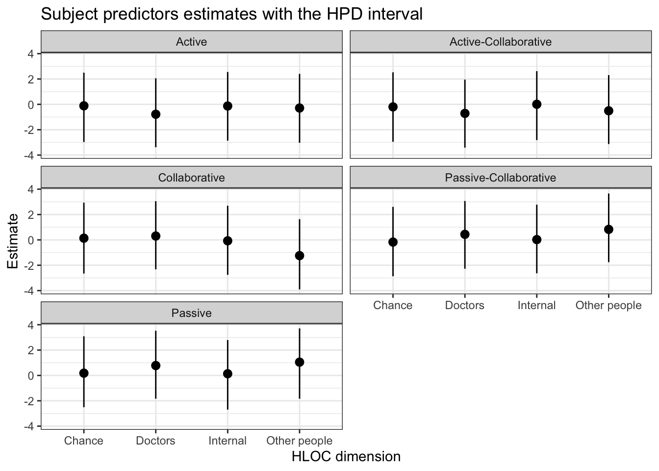

5.6.4 Probability tables

First let’s create a data frame with the cases we want to investigate. We will utilize the model_type option in the probabilities table so we can average out the values of the random effects in the subjects. In this table, we will only investigate a few of the conditions, but of course it is possible to do a much more expansive analysis

Let’s create a new data frame with the conditions we want to investigate. Mainly we are just investigating: * Between the choice of Active and Passive how does going from -2 to 2 standard deviations over the mean influences the probability in the Internal and the Doctors * Between the choice of Active-Collaborative and Collaborative how does going from -2 to 2 standard deviations over the mean influences the probability in the Internal and the Doctors * Between the choice of Collaborative and Passive-Collaborative how does going from -2 to 2 standard deviations over the mean influences the probability in the Internal and the Doctors

newdata <- tibble::tribble(~choice1, ~choice0, ~Internal, ~Chance, ~Doctors, ~OtherPeople,
                           "Active", "Passive", 0, 0, 0, 0,
                           "Active", "Passive", -2, 0, 0, 0,
                           "Active", "Passive", 2, 0, 0, 0,
                           "Active", "Passive", 0, 0, -2, 0,
                           "Active", "Passive", 0, 0, 2, 0,
                           "Active-Collaborative", "Collaborative", 0, 0, 0, 0,
                           "Active-Collaborative", "Collaborative", -2, 0, 0, 0,
                           "Active-Collaborative", "Collaborative", 2, 0, 0, 0,
                           "Active-Collaborative", "Collaborative", 0, 0, -2, 0,
                           "Active-Collaborative", "Collaborative", 0, 0, 2, 0,
                           "Collaborative", "Passive-Collaborative", 0, 0, 0, 0,
                           "Collaborative", "Passive-Collaborative", 0, -2, 0, 0,
                           "Collaborative", "Passive-Collaborative", 0, 2, 0, 0,
                           "Collaborative", "Passive-Collaborative", 0, 0, 0, -2,
                           "Collaborative", "Passive-Collaborative", 0, 0, 0, 2
                           )

#Now we can calculate the probabilities
prob_hloc <-
  get_probabilities_df(
    m3, 
    newdata = newdata,
    model_type = 'bt-subjectpredictors') #here we are assuming zero for the random effects

prob_hloc %>% 
  select(-j_beats_i) %>% 
  rename(Probability=i_beats_j) %>% 
  kable(caption = "Probabilities of selecting role i instead of j based on changes of the values of the HLOC dimensions",
      digits = 2,
      booktabs = T) %>% 
  kableExtra::kable_styling(bootstrap_options = c("striped", "hover", "condensed", "responsive")) %>% 
  kableExtra::add_header_above(c("Roles" = 2, "HLOC dimensions" = 4, " "=1)) %>% 
  kableExtra::scroll_box(width = "100%")

Table 5.4: Probabilities of selecting role i instead of j based on changes of the values of the HLOC dimensions
Roles		HLOC dimensions
i	j	Internal	Chance	Doctors	OtherPeople	Probability
Active	Passive	0	0	0	0	0.87
Active	Passive	-2	0	0	0	0.89
Active	Passive	2	0	0	0	0.86
Active	Passive	0	0	-2	0	0.84
Active	Passive	0	0	2	0	0.88
Active-Collaborative	Collaborative	0	0	0	0	0.07
Active-Collaborative	Collaborative	-2	0	0	0	0.07
Active-Collaborative	Collaborative	2	0	0	0	0.07
Active-Collaborative	Collaborative	0	0	-2	0	0.04
Active-Collaborative	Collaborative	0	0	2	0	0.07
Collaborative	Passive-Collaborative	0	0	0	0	0.98
Collaborative	Passive-Collaborative	0	-2	0	0	0.97
Collaborative	Passive-Collaborative	0	2	0	0	0.98
Collaborative	Passive-Collaborative	0	0	0	-2	0.96
Collaborative	Passive-Collaborative	0	0	0	2	0.95

5.7 Assessing fitness of items and judges

For simplification we will be using only the median (and not the full posterior) to assess the fitness of judges

std_judges <- U_std$Median #variance of the judges

U <- get_parameters(m3, params = 'U1', n_eff = T)
U_median <- U$Median
U_median <- U_median[-length(U_median)]

U_fit <- data.frame(U=U_median, y=rep(0,length(U_median)), q90=as.factor(as.numeric(U_median > std_judges*1.65)), q95=as.factor(as.numeric(U_median > std_judges*1.96)))

ggplot(data=U_fit, aes(x=U, y=y, color=q90))+
  geom_jitter() +
  geom_vline(xintercept = c(-1.65*std_judges,1.65*3), linetype = "dashed", color="red")+
  geom_vline(xintercept = c(-1.95*std_judges,1.95*3), linetype = "dashed", color="cyan")+
  theme(legend.position="none", axis.title.y = element_blank()) #small adjustments to the theme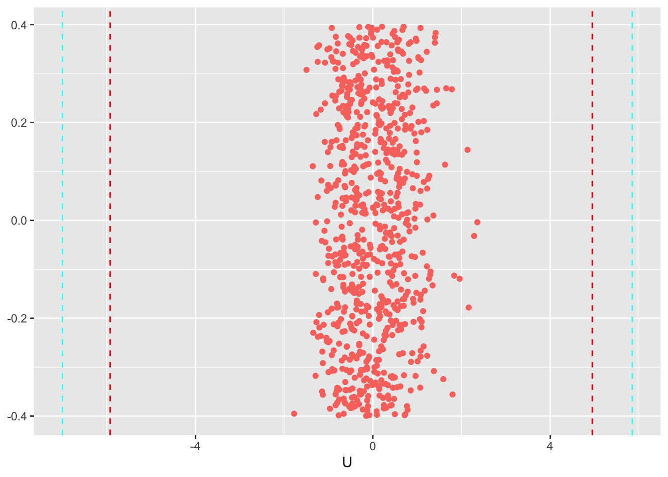

From this figure we can see that none of the judges rated a value outside the 90% and the 95% interval

Comparing to the prior distribution (with std of 3.0)

ggplot(data=U_fit, aes(x=U, y=y, color=q90))+
  geom_jitter() +
  geom_vline(xintercept = c(-1.65*3,1.65*3), linetype = "dashed", color="red")+
  geom_vline(xintercept = c(-1.95*3,1.95*3), linetype = "dashed", color="cyan")+
  theme(legend.position="none", axis.title.y = element_blank()) #small adjustments to the theme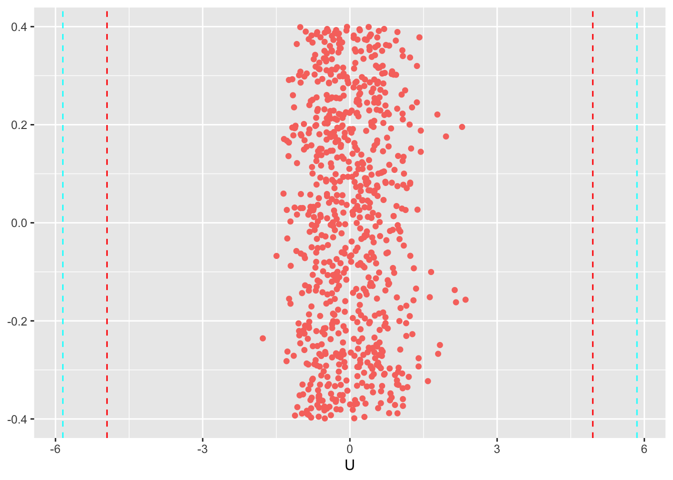

Finally we can look also if any of the judges can be considered to be outliers

Let’s use a Hample filter on the median values

lower_bound <- median(U_median) - 3 * mad(U_median, constant = 1)
upper_bound <- median(U_median) + 3 * mad(U_median, constant = 1)
which(U_median< lower_bound | U_median > upper_bound)

##  [1]  50 165 260 398 410 480 560 565 570 574 610 685

Within the values we have a few pairs of judges/items to be consider outliers, although without a misfit in terms of model

AB	AC	BC	AD	BD	CD	AE	BE	CE	DE	GENDER	MHLC_INTERNAL	MHLC_CHANCE	MHLC_DOCTORS	MHLC_OTHER_PEOPLE	Age
1	1	1	1	1	1	1	1	1	1	2	16	14	12	10	56
1	1	1	1	1	0	0	0	0	0	2	23	13	14	7	53
1	1	1	0	0	0	0	0	0	0	1	19	6	9	5	58
1	1	1	1	1	0	1	0	0	0	2	19	7	7	8	27
1	1	1	1	0	0	0	0	0	0	1	14	12	11	5	28

GENDER	MHLC_INTERNAL	MHLC_CHANCE	MHLC_DOCTORS	MHLC_OTHER_PEOPLE	Age	SubjectID	comparison	y	choice0	choice1
1	22	6	15	14	31	96	BE	1	B	E
2	20	17	8	9	26	125	DE	0	D	E
2	30	30	15	15	27	116	AC	1	A	C
2	23	8	14	9	55	36	BE	1	B	E
2	23	18	13	11	53	42	CD	0	C	D
1	20	17	14	9	37	79	AB	1	A	B
2	21	23	13	11	78	2	DE	0	D	E
2	20	23	8	13	30	100	CD	1	C	D
2	19	19	17	9	34	93	AE	1	A	E
2	33	31	8	13	45	58	DE	1	D	E

AB	AC	BC	AD	BD	CD	AE	BE	CE	DE	GENDER	MHLC_INTERNAL	MHLC_CHANCE	MHLC_DOCTORS	MHLC_OTHER_PEOPLE	Age
1	1	1	1	1	1	1	1	1	1	2	16	14	12	10	56
1	1	1	1	1	0	0	0	0	0	2	23	13	14	7	53
1	1	1	0	0	0	0	0	0	0	1	19	6	9	5	58
1	1	1	1	1	0	1	0	0	0	2	19	7	7	8	27
1	1	1	1	0	0	0	0	0	0	1	14	12	11	5	28

GENDER	MHLC_INTERNAL	MHLC_CHANCE	MHLC_DOCTORS	MHLC_OTHER_PEOPLE	Age	SubjectID	comparison	y	choice0	choice1
1	22	6	15	14	31	96	BE	1	B	E
2	20	17	8	9	26	125	DE	0	D	E
2	30	30	15	15	27	116	AC	1	A	C
2	23	8	14	9	55	36	BE	1	B	E
2	23	18	13	11	53	42	CD	0	C	D
1	20	17	14	9	37	79	AB	1	A	B
2	21	23	13	11	78	2	DE	0	D	E
2	20	23	8	13	30	100	CD	1	C	D
2	19	19	17	9	34	93	AE	1	A	E
2	33	31	8	13	45	58	DE	1	D	E

AB	AC	BC	AD	BD	CD	AE	BE	CE	DE	GENDER	MHLC_INTERNAL	MHLC_CHANCE	MHLC_DOCTORS	MHLC_OTHER_PEOPLE	Age
1	1	1	1	1	1	1	1	1	1	2	16	14	12	10	56
1	1	1	1	1	0	0	0	0	0	2	23	13	14	7	53
1	1	1	0	0	0	0	0	0	0	1	19	6	9	5	58
1	1	1	1	1	0	1	0	0	0	2	19	7	7	8	27
1	1	1	1	0	0	0	0	0	0	1	14	12	11	5	28

GENDER	MHLC_INTERNAL	MHLC_CHANCE	MHLC_DOCTORS	MHLC_OTHER_PEOPLE	Age	SubjectID	comparison	y	choice0	choice1
1	22	6	15	14	31	96	BE	1	B	E
2	20	17	8	9	26	125	DE	0	D	E
2	30	30	15	15	27	116	AC	1	A	C
2	23	8	14	9	55	36	BE	1	B	E
2	23	18	13	11	53	42	CD	0	C	D
1	20	17	14	9	37	79	AB	1	A	B
2	21	23	13	11	78	2	DE	0	D	E
2	20	23	8	13	30	100	CD	1	C	D
2	19	19	17	9	34	93	AE	1	A	E
2	33	31	8	13	45	58	DE	1	D	E