Chapter 3 Re-analysis 1

This reanalysis is based on the paper:

Iwasa, Kazunori, et al. “Visual perception of moisture is a pathogen detection mechanism of the behavioral immune system.” Frontiers in Psychology 11 (2020): 170.

The data of this paper can be obtained from the repository: https://osf.io/5quj9/

library(bpcs)
library(tidyverse)
library(knitr)
library(cmdstanr)
PATH_TO_CMDSTAN <- paste(Sys.getenv("HOME"), '/.cmdstan/cmdstan-2.27.0', sep = '')
set_cmdstan_path(PATH_TO_CMDSTAN)
set.seed(99)

3.1 Importing the data

First let’s read the data:

d <- readxl::read_xlsx('data/moisture.xlsx', sheet = 'Exp02_BTmodel')

Below we show a sample of how the original data looks like:

sample_n(d, size = 5) %>% 
  kable(caption = 'Sample of the original data') %>% 
  kableExtra::scroll_box(width = "100%")

Table 3.1: Sample of the original data

player1	player2	win1	win2
image7	image6	131	109
image5	image6	18	222
image7	image2	226	14
image4	image1	239	1
image5	image8	20	220

The data is in the aggregated format. So let’s expand it to the long format

d_moisture <- expand_aggregated_data(d, player0 = 'player1', player1='player2', wins0 = 'win1', wins1='win2')

Now the data looks like this:

sample_n(d_moisture, size = 20) %>% 
  kable(caption = 'The data in the long format') %>% 
  kableExtra::scroll_box(width = "100%")

Table 3.2: The data in the long format

player0	player1	y	rowid
image2	image7	1	2922
image5	image2	0	7102
image7	image6	1	11490
image2	image8	1	3200
image1	image3	1	358
image8	image4	1	12704
image6	image3	0	8973
image8	image3	0	12308
image6	image4	0	9188
image5	image2	0	7071
image5	image1	0	6724
image4	image7	1	6409
image8	image1	0	11986
image4	image1	0	5278
image3	image7	1	4694
image4	image5	1	5972
image1	image8	1	1533
image4	image8	1	6560
image1	image3	1	398
image3	image5	1	4228

3.2 Analysis with the Bradley-Terry model and the order effect model

Although this is multiple judgment case, the dataset in the aggregated format does not provide information of how each individual voted, therefore we cannot compensate this effect. Therefore, we will create an analysis with only the Bradley-Terry model and the Bradley-Terry model with order effect

First, let’s sample the Bradley-Terry model

m_moisture <-
  bpc(
    d_moisture,
    player0 = 'player0',
    player1 = 'player1',
    result_column = 'y',
    model_type = 'bt',
    iter = 2000,
    show_chain_messages = T
  )
save_bpc_model(m_moisture,'m_moisture','./fittedmodels')

Low let’s sample the model with order effect.

Although the authors said that the order of the images was inverted to compensate order effect, we can still estimate if there is an order effect or not in the choice.

But first we need to create a column indicating if there was order effect for that case or not. In this problem, we just indicate with a column of ones that all instances could have an order effect. Not that the package marks the order effect relative to player1. So if the values should be interpret as such.

d_moisture <- d_moisture %>% 
  dplyr::mutate(z1 = 1)

m_moisture_order <-
  bpc(
    d_moisture,
    player0 = 'player0',
    player1 = 'player1',
    result_column = 'y',
    z_player1 = 'z1',
    model_type = 'bt-ordereffect',
    iter = 2000,
    show_chain_messages = T
  )
save_bpc_model(m_moisture_order,'m_moisture_order','./fittedmodels')

3.3 Diagnostics

check_convergence_diagnostics(m_moisture)

## Processing csv files: /Users/xramor/OneDrive/2021/bpcs-online-appendix/.bpcs/bt-202109130836-1-55f37e.csv, /Users/xramor/OneDrive/2021/bpcs-online-appendix/.bpcs/bt-202109130836-2-55f37e.csv, /Users/xramor/OneDrive/2021/bpcs-online-appendix/.bpcs/bt-202109130836-3-55f37e.csv, /Users/xramor/OneDrive/2021/bpcs-online-appendix/.bpcs/bt-202109130836-4-55f37e.csv
## 
## Checking sampler transitions treedepth.
## Treedepth satisfactory for all transitions.
## 
## Checking sampler transitions for divergences.
## No divergent transitions found.
## 
## Checking E-BFMI - sampler transitions HMC potential energy.
## E-BFMI satisfactory.
## 
## Effective sample size satisfactory.
## 
## Split R-hat values satisfactory all parameters.
## 
## Processing complete, no problems detected.

check_convergence_diagnostics(m_moisture_order)

## Processing csv files: /Users/xramor/OneDrive/2021/bpcs-online-appendix/.bpcs/bt-202109130912-1-1cedf9.csv, /Users/xramor/OneDrive/2021/bpcs-online-appendix/.bpcs/bt-202109130912-2-1cedf9.csv, /Users/xramor/OneDrive/2021/bpcs-online-appendix/.bpcs/bt-202109130912-3-1cedf9.csv, /Users/xramor/OneDrive/2021/bpcs-online-appendix/.bpcs/bt-202109130912-4-1cedf9.csv
## 
## Checking sampler transitions treedepth.
## Treedepth satisfactory for all transitions.
## 
## Checking sampler transitions for divergences.
## No divergent transitions found.
## 
## Checking E-BFMI - sampler transitions HMC potential energy.
## E-BFMI satisfactory.
## 
## Effective sample size satisfactory.
## 
## Split R-hat values satisfactory all parameters.
## 
## Processing complete, no problems detected.

Checking convergence of the models with shinystan

launch_shinystan(m_moisture)

launch_shinystan(m_moisture_order)

3.3.1 Tables and plots

First, lets get a table for the parameters (to export it to Latex just utilize the format option)

get_parameters_table(m_moisture, format = 'html', caption = 'Parameters estimates for the simple Bradley-Terry model')

Table 3.3: Parameters estimates for the simple Bradley-Terry model

Parameter	Mean	Median	HPD_lower	HPD_higher
lambda[image1]	-4.476	-4.492	-6.800	-2.407
lambda[image2]	-2.362	-2.379	-4.680	-0.298
lambda[image3]	-0.049	-0.067	-2.408	1.986
lambda[image4]	0.144	0.126	-2.095	2.302
lambda[image5]	0.303	0.283	-1.916	2.476
lambda[image6]	1.848	1.826	-0.409	3.980
lambda[image7]	2.023	2.002	-0.210	4.193
lambda[image8]	3.038	3.014	0.642	5.052

get_parameters_table(
  m_moisture_order,
  params = c('lambda', 'gm'),
  format = 'html',
  caption = 'Parameters estimates for the Bradley-Terry model with order effect',
  keep_par_name = F,
  n_eff = T
)

Table 3.4: Parameters estimates for the Bradley-Terry model with order effect

Parameter	Mean	Median	HPD_lower	HPD_higher	n_eff
image1	-4.525	-4.560	-6.616	-2.522	843
image2	-2.413	-2.453	-4.513	-0.424	842
image3	-0.101	-0.141	-2.152	1.924	842
image4	0.091	0.048	-2.009	2.080	841
image5	0.251	0.216	-1.797	2.287	841
image6	1.795	1.755	-0.289	3.798	838
image7	1.970	1.931	-0.146	3.940	836
image8	2.984	2.952	0.943	5.035	841
gm	0.001	0.001	-0.054	0.058	1825

We can see from the table of the order effect that the gamma parameter is very close to zero, indicating that there is no order effect

Now lets compute the posterior ranks of the images based on the first BT model

r <- get_rank_of_players_df(m_moisture) 

Generating a table with the images

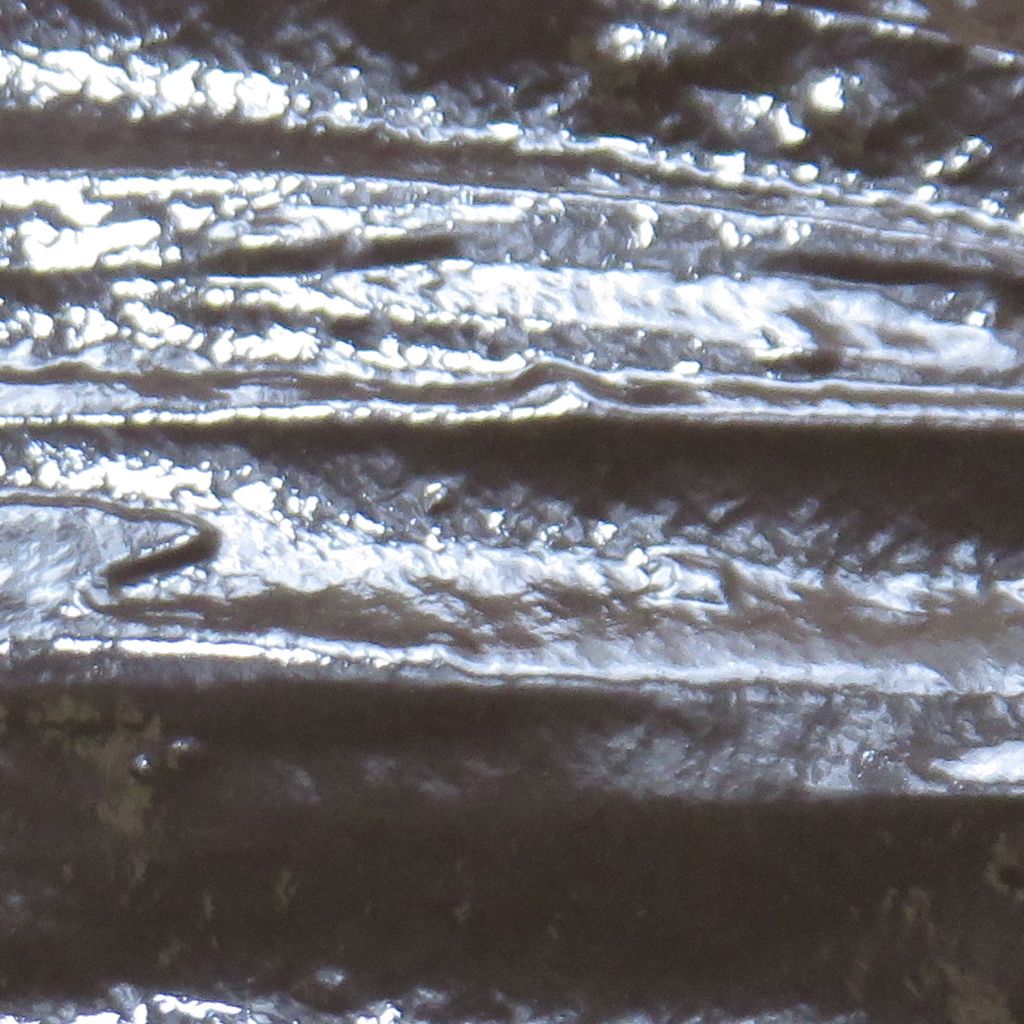
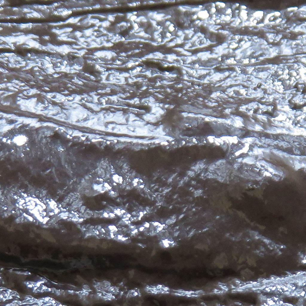
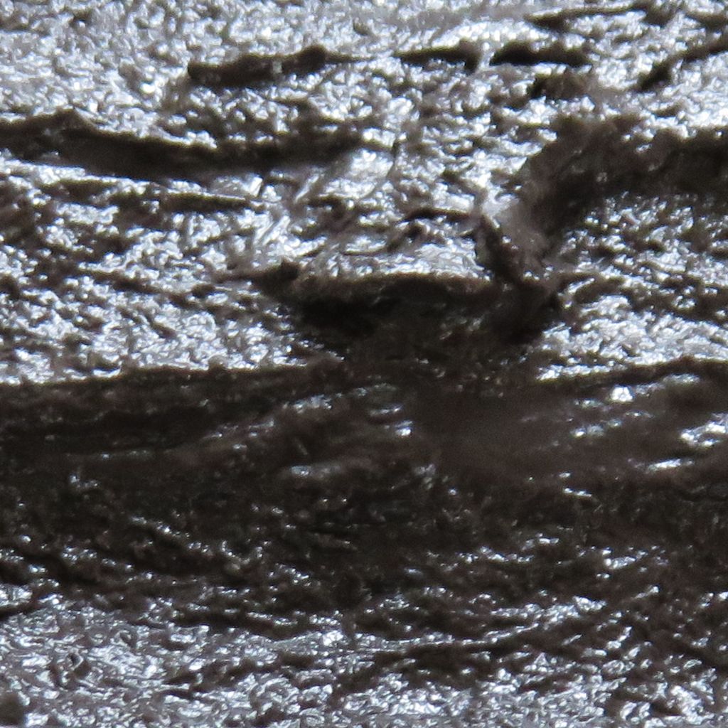
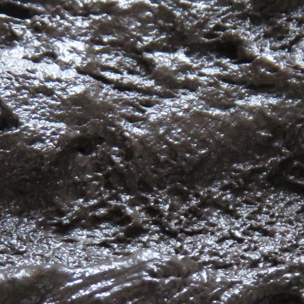
r %>% 
  mutate(Image = c("data/moisture/Stimuli/image08.jpg",
                   "data/moisture/Stimuli/image07.jpg",
                   "data/moisture/Stimuli/image06.jpg",
                   "data/moisture/Stimuli/image05.jpg",
                   "data/moisture/Stimuli/image04.jpg",
                   "data/moisture/Stimuli/image03.jpg",
                   "data/moisture/Stimuli/image02.jpg",
                   "data/moisture/Stimuli/image01.jpg") %>% pander::pandoc.image.return()) %>% 
  knitr::kable(caption = "Rank of the images based on moisture content", format='html', booktabs=T)

Table 3.5: Rank of the images based on moisture content

Parameter	MedianRank	MeanRank	StdRank	Image
image8	1	1.000	0.0000000
image7	2	2.002	0.0446990
image6	3	2.998	0.0446990
image5	4	4.006	0.0772656
image4	5	4.995	0.0835583
image3	6	5.999	0.0316228
image2	7	7.000	0.0000000
image1	8	8.000	0.0000000

Now lets get a caterpillar style plot

plot(
  m_moisture_order,
  HPDI = T,
  title = 'Estimates of the moisture content',
  xaxis = 'Images',
  yaxis = 'Ability',
  rotate_x_labels = F,
  APA = F,
  keep_par_names=F) + theme_bw()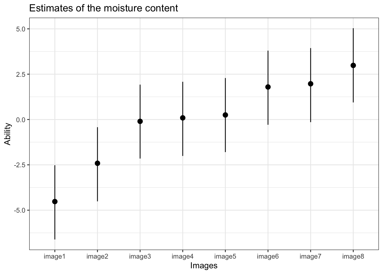

3.3.2 WAIC

Calculating the WAIC of both models

get_waic(m_moisture)

## 
## Computed from 8000 by 13440 log-likelihood matrix
## 
##           Estimate    SE
## elpd_waic  -4066.2  78.9
## p_waic         7.0   0.2
## waic        8132.4 157.7

get_waic(m_moisture_order)

## 
## Computed from 8000 by 13440 log-likelihood matrix
## 
##           Estimate    SE
## elpd_waic  -4067.2  78.8
## p_waic         7.9   0.2
## waic        8134.3 157.7

We can see that the WAIC of the models are quite similar and that the model without the order effect has a slightly smaller WAIC and less parameters. Therefore we will select it.