Chapter 4 Re-analysis 2

This reanalysis is based on the paper:

Huskisson, S.M., Jacobson, S.L., Egelkamp, C.L. et al. Using a Touchscreen Paradigm to Evaluate Food Preferences and Response to Novel Photographic Stimuli of Food in Three Primate Species (Gorilla gorilla gorilla, Pan troglodytes, and Macaca fuscata). Int J Primatol 41, 5–23 (2020). https://doi.org/10.1007/s10764-020-00131-0

library(bpcs)
library(tidyverse)
library(knitr)
library(cmdstanr)
PATH_TO_CMDSTAN <- paste(Sys.getenv("HOME"), '/.cmdstan/cmdstan-2.27.0', sep = '')
set_cmdstan_path(PATH_TO_CMDSTAN)
set.seed(99)

4.1 Importing the data

The data from this paper was made available upon request and below we exemplify a few rows of how the original dataset looks like

d <- readr::read_csv('data/touchscreen.csv')

Previewing how the data looks like

dplyr::sample_n(d, size = 10) %>% 
  knitr::kable(caption='Sample of how the dataset looks like') %>% 
  kableExtra::kable_styling(bootstrap_options = c("striped", "hover", "condensed", "responsive")) %>% 
  kableExtra::scroll_box(width = "100%")

Table 4.1: Sample of how the dataset looks like
date	species_type	SubjectCode	Sex	Trial	image1	image2	image_chosen	concat_test_name
10/12/17	Gorilla	Gorilla1	Male	2	Ap	Cu	Ap	ApCu
8/31/17	Gorilla	Gorilla3	Male	16	Ca	To	To	CaTo
8/16/17	Gorilla	Gorilla5	Female	16	Cu	Gr	Cu	CuGr
11/13/17	Chimpanzee	Chimpanzee3	Female	14	Ap	Ca	Ca	ApCa
4/11/17	Gorilla	Gorilla3	Male	15	Ca	Cu	Ca	CaCu
1/22/18	Macaque	Macaque7	Female	1	Ca	Pe	Pe	CaPe
1/5/17	Gorilla	Gorilla4	Male	28	Ca	Tu	Tu	CaTu
3/3/17	Chimpanzee	Chimpanzee1	Female	19	Cu	Gr	Gr	CuGr
12/4/17	Chimpanzee	Chimpanzee1	Female	27	Ap	Tu	Tu	ApTu
5/1/17	Gorilla	Gorilla6	Male	14	Ca	Tu	Ca	CaTu

Now we need to modify a bit the data frame to create a column with the results as 0 and 1.

Creating a numerical result vector with 0 for image1 and 1 for image2

d <- d %>% 
  dplyr::mutate(y =ifelse(image_chosen==image1, 0, 1))

Adding names to the abbreviations

#image1
d$image1 <- dplyr::recode(d$image1, "Ca" = 'Carrot')
d$image1 <- dplyr::recode(d$image1, "Cu" = 'Cucumber')
d$image1 <- dplyr::recode(d$image1, "Tu" = 'Turnip')
d$image1 <- dplyr::recode(d$image1, "Gr" = 'Grape')
d$image1 <- dplyr::recode(d$image1, "To" = 'Tomato')
d$image1 <- dplyr::recode(d$image1, "Ap" = 'Apple')
d$image1 <- dplyr::recode(d$image1, "Jp" = 'Jungle Pellet')
d$image1 <- dplyr::recode(d$image1, "Ce" = 'Celery')
d$image1 <- dplyr::recode(d$image1, "Gb" = 'Green Beans')
d$image1 <- dplyr::recode(d$image1, "Oa" = 'Oats')
d$image1 <- dplyr::recode(d$image1, "Pe" = 'Peanuts')

#image2
d$image2 <- dplyr::recode(d$image2, "Ca" = 'Carrot')
d$image2 <- dplyr::recode(d$image2, "Cu" = 'Cucumber')
d$image2 <- dplyr::recode(d$image2, "Tu" = 'Turnip')
d$image2 <- dplyr::recode(d$image2, "Gr" = 'Grape')
d$image2 <- dplyr::recode(d$image2, "To" = 'Tomato')
d$image2 <- dplyr::recode(d$image2, "Ap" = 'Apple')
d$image2 <- dplyr::recode(d$image2, "Jp" = 'Jungle Pellet')
d$image2 <- dplyr::recode(d$image2, "Ce" = 'Celery')
d$image2 <- dplyr::recode(d$image2, "Gb" = 'Green Beans')
d$image2 <- dplyr::recode(d$image2, "Oa" = 'Oats')
d$image2 <- dplyr::recode(d$image2, "Pe" = 'Peanuts')

Separating the data into three datasets. One for each species.

macaque <- d %>% 
  dplyr::filter(species_type=='Macaque')

chip <- d %>% 
  dplyr::filter(species_type=='Chimpanzee')

gor <- d %>% 
  dplyr::filter(species_type=='Gorilla')

Below we show a few lines of each dataset:

dplyr::sample_n(gor, size = 10) %>% 
  knitr::kable(caption='Sample of how the gorilla dataset looks like') %>% 
  kableExtra::kable_styling(bootstrap_options = c("striped", "hover", "condensed", "responsive")) %>% 
  kableExtra::scroll_box(width = "100%")

Table 4.2: Sample of how the gorilla dataset looks like
date	species_type	SubjectCode	Sex	Trial	image1	image2	image_chosen	concat_test_name	y
3/3/17	Gorilla	Gorilla2	Male	31	Cucumber	Tomato	To	CuTo	1
11/8/17	Gorilla	Gorilla6	Male	6	Tomato	Turnip	To	ToTu	0
3/20/17	Gorilla	Gorilla2	Male	6	Grape	Tomato	To	GrTo	1
3/8/17	Gorilla	Gorilla6	Male	20	Carrot	Grape	Ca	CaGr	0
8/23/17	Gorilla	Gorilla5	Female	4	Cucumber	Grape	Cu	CuGr	0
5/25/17	Gorilla	Gorilla4	Male	19	Carrot	Cucumber	Ca	CaCu	0
8/3/17	Gorilla	Gorilla6	Male	14	Carrot	Tomato	To	CaTo	1
8/23/17	Gorilla	Gorilla5	Female	24	Cucumber	Grape	Gr	CuGr	1
12/7/16	Gorilla	Gorilla2	Male	28	Cucumber	Turnip	Cu	CuTu	0
5/25/17	Gorilla	Gorilla1	Male	4	Carrot	Cucumber	Ca	CaCu	0

dplyr::sample_n(chip, size = 10) %>% 
  knitr::kable(caption='Sample of how the chimpanzees dataset looks like') %>% 
  kableExtra::kable_styling(bootstrap_options = c("striped", "hover", "condensed", "responsive")) %>% 
  kableExtra::scroll_box(width = "100%")

Table 4.3: Sample of how the chimpanzees dataset looks like
date	species_type	SubjectCode	Sex	Trial	image1	image2	image_chosen	concat_test_name	y
3/1/18	Chimpanzee	Chimpanzee4	Male	3	Apple	Carrot	Ap	ApCa	0
12/7/17	Chimpanzee	Chimpanzee1	Female	18	Carrot	Tomato	To	CaTo	1
4/26/17	Chimpanzee	Chimpanzee3	Female	7	Cucumber	Turnip	Cu	CuTu	0
11/1/17	Chimpanzee	Chimpanzee1	Female	19	Apple	Grape	Gr	ApGr	1
7/26/17	Chimpanzee	Chimpanzee3	Female	20	Cucumber	Grape	Cu	CuGr	0
10/26/17	Chimpanzee	Chimpanzee1	Female	7	Apple	Grape	Gr	ApGr	1
9/18/17	Chimpanzee	Chimpanzee4	Male	27	Carrot	Grape	Gr	CaGr	1
12/8/16	Chimpanzee	Chimpanzee1	Female	12	Cucumber	Turnip	Cu	CuTu	0
12/14/17	Chimpanzee	Chimpanzee3	Female	14	Tomato	Turnip	To	ToTu	0
1/12/17	Chimpanzee	Chimpanzee4	Male	21	Cucumber	Turnip	Tu	CuTu	1

dplyr::sample_n(macaque, size = 10) %>% 
  knitr::kable(caption='Sample of how the macaques dataset looks like') %>% 
  kableExtra::kable_styling(bootstrap_options = c("striped", "hover", "condensed", "responsive")) %>% 
  kableExtra::scroll_box(width = "100%")

Table 4.4: Sample of how the macaques dataset looks like
date	species_type	SubjectCode	Sex	Trial	image1	image2	image_chosen	concat_test_name	y
10/6/17	Macaque	Macaque6	Female	10	Jungle Pellet	Celery	Jp	CeJp	0
09-06-2017@11-43	Macaque	Macaque1	Male	12	Carrot	Celery	Ca	CeCa	0
04-30-2018@11-54	Macaque	Macaque1	Male	8	Peanuts	Oats	Pe	PeOa	0
8/7/17	Macaque	Macaque3	Female	1	Peanuts	Celery	Ce	CePe	1
05-04-2018@11-27	Macaque	Macaque1	Male	1	Celery	Green Beans	Gb	GbCe	1
1/16/18	Macaque	Macaque7	Female	14	Carrot	Peanuts	Ca	CaPe	0
04-02-2018@11-27	Macaque	Macaque1	Male	28	Carrot	Green Beans	Ca	GbCa	0
9/7/17	Macaque	Macaque6	Female	2	Carrot	Celery	Ca	CeCa	0
8/14/17	Macaque	Macaque2	Female	14	Carrot	Peanuts	Pe	CaPe	1
5/24/18	Macaque	Macaque4	Female	17	Jungle Pellet	Oats	Jp	JpOa	0

4.2 Simple Bradley-Terry model

Now that the data is ready let’s fit three simple Bayesian Bradley-Terry models

m1_macaque <-
  bpc(
    macaque,
    player0 = 'image1',
    player1 = 'image2',
    result_column = 'y',
    model_type = 'bt',
    priors = list(prior_lambda_std = 3.0),
    iter = 3000,
    show_chain_messages = T
  )
save_bpc_model(m1_macaque, 'm1_macaque', './fittedmodels')

m1_chip <-
  bpc(
    chip,
    player0 = 'image1',
    player1 = 'image2',
    result_column = 'y',
    model_type = 'bt',
    priors = list(prior_lambda_std = 3.0),
    iter = 3000,
    show_chain_messages = T
  )
save_bpc_model(m1_chip, 'm1_chip', './fittedmodels')

m1_gor <-
  bpc(
    gor,
    player0 = 'image1',
    player1 = 'image2',
    result_column = 'y',
    model_type = 'bt',
    priors = list(prior_lambda_std = 3.0),
    iter = 3000,
    show_chain_messages = T
  )
save_bpc_model(m1_gor, 'm1_gor', './fittedmodels')

4.2.1 Assessing the fitness of the model

Here we are illustrating how to conduct the diagnostic analysis for one model only. Since the shinystan app does not appear in the compiled appendix we are just representing it here once for the Chimpanzees model. Note that it is still possible to use the bayesplot package to generate static figures if needed.

#First we get the posterior predictive in the environment
pp_m1_chip <- posterior_predictive(m1_chip, n = 100)
y_pp_m1_chip <- pp_m1_chip_gor$y
ypred_pp_m1_chip <- pp_m1_chip$y_pred

Then we launch shinystan to assess convergence and validity of the model (e.g.)

launch_shinystan(m1_chip)

We can also do some quick checks with:

check_convergence_diagnostics(m1_chip)

## Processing csv files: /Users/xramor/OneDrive/2021/bpcs-online-appendix/.bpcs/bt-202109131150-1-43ae25.csv, /Users/xramor/OneDrive/2021/bpcs-online-appendix/.bpcs/bt-202109131150-2-43ae25.csv, /Users/xramor/OneDrive/2021/bpcs-online-appendix/.bpcs/bt-202109131150-3-43ae25.csv, /Users/xramor/OneDrive/2021/bpcs-online-appendix/.bpcs/bt-202109131150-4-43ae25.csv
## 
## Checking sampler transitions treedepth.
## Treedepth satisfactory for all transitions.
## 
## Checking sampler transitions for divergences.
## No divergent transitions found.
## 
## Checking E-BFMI - sampler transitions HMC potential energy.
## E-BFMI satisfactory.
## 
## Effective sample size satisfactory.
## 
## Split R-hat values satisfactory all parameters.
## 
## Processing complete, no problems detected.

check_convergence_diagnostics(m1_macaque)

## Processing csv files: /Users/xramor/OneDrive/2021/bpcs-online-appendix/.bpcs/bt-202109131120-1-5538ef.csv, /Users/xramor/OneDrive/2021/bpcs-online-appendix/.bpcs/bt-202109131120-2-5538ef.csv, /Users/xramor/OneDrive/2021/bpcs-online-appendix/.bpcs/bt-202109131120-3-5538ef.csv, /Users/xramor/OneDrive/2021/bpcs-online-appendix/.bpcs/bt-202109131120-4-5538ef.csv
## 
## Checking sampler transitions treedepth.
## Treedepth satisfactory for all transitions.
## 
## Checking sampler transitions for divergences.
## No divergent transitions found.
## 
## Checking E-BFMI - sampler transitions HMC potential energy.
## E-BFMI satisfactory.
## 
## Effective sample size satisfactory.
## 
## Split R-hat values satisfactory all parameters.
## 
## Processing complete, no problems detected.

check_convergence_diagnostics(m1_gor)

## Processing csv files: /Users/xramor/OneDrive/2021/bpcs-online-appendix/.bpcs/bt-202109131238-1-8085bd.csv, /Users/xramor/OneDrive/2021/bpcs-online-appendix/.bpcs/bt-202109131238-2-8085bd.csv, /Users/xramor/OneDrive/2021/bpcs-online-appendix/.bpcs/bt-202109131238-3-8085bd.csv, /Users/xramor/OneDrive/2021/bpcs-online-appendix/.bpcs/bt-202109131238-4-8085bd.csv
## 
## Checking sampler transitions treedepth.
## Treedepth satisfactory for all transitions.
## 
## Checking sampler transitions for divergences.
## No divergent transitions found.
## 
## Checking E-BFMI - sampler transitions HMC potential energy.
## E-BFMI satisfactory.
## 
## Effective sample size satisfactory.
## 
## Split R-hat values satisfactory all parameters.
## 
## Processing complete, no problems detected.

4.2.2 Getting the WAIC

Before we start getting the parameters tables and etc let’s get the WAIC so we can compare with the next model (with random effects)

get_waic(m1_macaque)

## 
## Computed from 12000 by 8400 log-likelihood matrix
## 
##           Estimate    SE
## elpd_waic  -3550.7  56.9
## p_waic         5.0   0.1
## waic        7101.4 113.8

get_waic(m1_chip)

## 
## Computed from 12000 by 5400 log-likelihood matrix
## 
##           Estimate   SE
## elpd_waic  -3599.7 17.0
## p_waic         5.0  0.0
## waic        7199.4 34.0

get_waic(m1_gor)

## 
## Computed from 12000 by 8100 log-likelihood matrix
## 
##           Estimate   SE
## elpd_waic  -4883.7 36.0
## p_waic         5.0  0.1
## waic        9767.3 72.0

4.3 Bradley-Terry model with random effects for individuals

Let’s add the cluster SubjectCode as a random effects in our model

m2_macaque <-
  bpc(
    macaque,
    player0 = 'image1',
    player1 = 'image2',
    result_column = 'y',
    model_type = 'bt-U',
    cluster = c('SubjectCode'),
    priors = list(
      prior_lambda_std = 1.0,
      prior_U1_std = 1.0
    ),
    iter = 3000,
    show_chain_messages = T
  )
save_bpc_model(m2_macaque, 'm2_macaque', './fittedmodels')

m2_chip <-
  bpc(
    chip,
    player0 = 'image1',
    player1 = 'image2',
    cluster = c('SubjectCode'),
    result_column = 'y',
    model_type = 'bt-U',
    priors = list(
      prior_lambda_std = 1.0,
      prior_U1_std = 1.0
    ),
    iter = 3000,
    show_chain_messages = T
  )
save_bpc_model(m2_chip, 'm2_chip', './fittedmodels')

m2_gor <-
  bpc(
    gor,
    player0 = 'image1',
    player1 = 'image2',
    cluster = c('SubjectCode'),
    result_column = 'y',
    model_type = 'bt-U',
    priors = list(
      prior_lambda_std = 1.0,
      prior_U1_std = 1.0
    ),
    iter = 3000,
    show_chain_messages = T
  )
save_bpc_model(m2_gor, 'm2_gor', './fittedmodels')

Of course we should run diagnostic analysis on the models. For the gorillas

launch_shinystan(m2_gor)

We can also do some quick checks with:

check_convergence_diagnostics(m2_chip)

## Processing csv files: /Users/xramor/OneDrive/2021/bpcs-online-appendix/.bpcs/bt-202109131533-1-7cb3c6.csv, /Users/xramor/OneDrive/2021/bpcs-online-appendix/.bpcs/bt-202109131533-2-7cb3c6.csv, /Users/xramor/OneDrive/2021/bpcs-online-appendix/.bpcs/bt-202109131533-3-7cb3c6.csv, /Users/xramor/OneDrive/2021/bpcs-online-appendix/.bpcs/bt-202109131533-4-7cb3c6.csv
## 
## Checking sampler transitions treedepth.
## Treedepth satisfactory for all transitions.
## 
## Checking sampler transitions for divergences.
## No divergent transitions found.
## 
## Checking E-BFMI - sampler transitions HMC potential energy.
## E-BFMI satisfactory.
## 
## Effective sample size satisfactory.
## 
## Split R-hat values satisfactory all parameters.
## 
## Processing complete, no problems detected.

check_convergence_diagnostics(m2_macaque)

## Processing csv files: /Users/xramor/OneDrive/2021/bpcs-online-appendix/.bpcs/bt-202109131424-1-46c43b.csv, /Users/xramor/OneDrive/2021/bpcs-online-appendix/.bpcs/bt-202109131424-2-46c43b.csv, /Users/xramor/OneDrive/2021/bpcs-online-appendix/.bpcs/bt-202109131424-3-46c43b.csv, /Users/xramor/OneDrive/2021/bpcs-online-appendix/.bpcs/bt-202109131424-4-46c43b.csv
## 
## Checking sampler transitions treedepth.
## Treedepth satisfactory for all transitions.
## 
## Checking sampler transitions for divergences.
## No divergent transitions found.
## 
## Checking E-BFMI - sampler transitions HMC potential energy.
## E-BFMI satisfactory.
## 
## Effective sample size satisfactory.
## 
## Split R-hat values satisfactory all parameters.
## 
## Processing complete, no problems detected.

check_convergence_diagnostics(m2_gor)

## Processing csv files: /Users/xramor/OneDrive/2021/bpcs-online-appendix/.bpcs/bt-202109131624-1-574b12.csv, /Users/xramor/OneDrive/2021/bpcs-online-appendix/.bpcs/bt-202109131624-2-574b12.csv, /Users/xramor/OneDrive/2021/bpcs-online-appendix/.bpcs/bt-202109131624-3-574b12.csv, /Users/xramor/OneDrive/2021/bpcs-online-appendix/.bpcs/bt-202109131624-4-574b12.csv
## 
## Checking sampler transitions treedepth.
## Treedepth satisfactory for all transitions.
## 
## Checking sampler transitions for divergences.
## No divergent transitions found.
## 
## Checking E-BFMI - sampler transitions HMC potential energy.
## E-BFMI satisfactory.
## 
## Effective sample size satisfactory.
## 
## Split R-hat values satisfactory all parameters.
## 
## Processing complete, no problems detected.

4.3.1 Getting the WAIC

Before we start plotting tables let’s get the WAIC for each random effects model and compare with the first models without random effects

get_waic(m2_macaque)

## 
## Computed from 12000 by 8400 log-likelihood matrix
## 
##           Estimate    SE
## elpd_waic  -3356.3  57.1
## p_waic        32.6   0.8
## waic        6712.5 114.2

get_waic(m2_chip)

## 
## Computed from 12000 by 5400 log-likelihood matrix
## 
##           Estimate   SE
## elpd_waic  -3360.0 24.1
## p_waic        19.7  0.3
## waic        6720.0 48.3

get_waic(m2_gor)

## 
## Computed from 12000 by 8100 log-likelihood matrix
## 
##           Estimate   SE
## elpd_waic  -4396.3 40.1
## p_waic        29.4  0.4
## waic        8792.5 80.2

Below I just copied the result of the WAIC into a data frame to create the tables. Of course this process could be automated.

waic_table <-
  data.frame(
    Species = c('Macaques', 'Chimpanzees', 'Gorillas'),
    BT = c(7101.5, 7199.4, 9767.2),
    BTU = c(6712.6, 6720.0, 8792.9)
  )

The kableExtra package provides some nice tools to create tables from R directly to Latex

kable(
  waic_table,  booktabs=T,
  caption = 'Comparison of the WAIC of the Bradley-Terry model and the Bradley-Terry model with random effects on the subjects for each specie.',
  col.names = c('Specie', 'Bradley-Terry', 'Bradley-Terry with random effects')
) %>%
  kableExtra::add_header_above(c(" " = 1, "WAIC" = 2)) %>%
  kableExtra::kable_styling(bootstrap_options = c("striped", "hover", "condensed", "responsive")) %>% 
  kableExtra::scroll_box(width = "100%")

Table 4.5: Comparison of the WAIC of the Bradley-Terry model and the Bradley-Terry model with random effects on the subjects for each specie.
	WAIC
Specie	Bradley-Terry	Bradley-Terry with random effects
Macaques	7101.5	6712.6
Chimpanzees	7199.4	6720.0
Gorillas	9767.2	8792.9

We can see that the random effects model perform much better than the simple BT model by having a much lower WAIC. Therefore from now we will use only the random effects model to generate our tables and plots

4.3.2 Parameter tables and plots

Now let’s create some plots and tables to analyze and compare the models

4.3.2.1 Parameters table

Creating a nice table of the parameters.

First let’s put all species in the same data frame

df1 <- get_parameters(m2_macaque, n_eff = T, keep_par_name = F)
df2 <- get_parameters(m2_chip, n_eff = T, keep_par_name = F)
df3 <- get_parameters(m2_gor, n_eff = T, keep_par_name = F)

df1 <- df1 %>% dplyr::mutate(Species='Macaque')
df2 <- df2 %>% dplyr::mutate(Species='Chimpanzees')
df3 <- df3 %>% dplyr::mutate(Species='Gorilla')

#appending the dataframes
df <- rbind(df1,df2,df3)

#Removing the individual random effects parameters otherwise the table will be much bigger
df <- df %>% 
  filter(!startsWith(Parameter,'U1['))

rownames(df) <- NULL

Now let’s create the table by removing the species column and adding some row Headers for the species

(df %>% select(-Species) %>% 
kable( caption = 'Parameters of the random effects model with 95% HPD and the number of effective samples.', digits = 2, col.names = c('Parameter', 'Mean', 'Median', 'HPD lower', 'HPD upper', 'N. Eff. Samples'), row.names = NA) %>% 
kableExtra::kable_styling(bootstrap_options = c("striped", "hover", "condensed", "responsive")) %>% 
  kableExtra::pack_rows("Macaque", 1, 6) %>%
  kableExtra::pack_rows("Chimpanzees", 7, 13) %>% 
  kableExtra::pack_rows("Gorilla", 14, 20) %>% 
  kableExtra::scroll_box(width = "100%")
)

Table 4.6: Parameters of the random effects model with 95% HPD and the number of effective samples.
Parameter	Mean	Median	HPD lower	HPD upper	N. Eff. Samples
Macaque
Carrot	0.12	0.12	-0.78	1.01	8222
Celery	-2.27	-2.27	-3.21	-1.41	7928
Jungle Pellet	1.23	1.23	0.36	2.16	7772
Oats	-0.90	-0.89	-1.78	0.02	7856
Peanuts	2.01	2.01	1.09	2.88	7855
Green Beans	-0.17	-0.16	-1.08	0.70	8137
Chimpanzees
U1_std	0.58	0.57	0.42	0.76	4487
Apple	0.03	0.03	-1.01	1.04	11102
Tomato	0.33	0.33	-0.71	1.30	11361
Carrot	-0.21	-0.21	-1.19	0.83	11334
Grape	0.61	0.62	-0.37	1.66	11549
Cucumber	-0.32	-0.32	-1.31	0.73	11198
Turnip	-0.43	-0.43	-1.42	0.59	11066
Gorilla
U1_std	0.72	0.70	0.48	1.00	4933
Apple	0.03	0.03	-0.93	1.01	13610
Carrot	-0.11	-0.11	-1.07	0.91	13400
Grape	0.87	0.88	-0.14	1.85	14689
Tomato	0.86	0.87	-0.11	1.82	12715
Cucumber	-0.70	-0.71	-1.74	0.23	13831
Turnip	-0.94	-0.94	-1.92	0.04	13596
U1_std	0.78	0.77	0.56	1.03	4943

4.3.2.2 Rank table

Rank of the food preferences

rank1 <- get_rank_of_players_df(m2_macaque)
rank2 <- get_rank_of_players_df(m2_chip)
rank3 <- get_rank_of_players_df(m2_gor)

#appending the dataframes
rank_all <- rbind(rank1,rank2,rank3)

Now let’s create the rank table

(rank_all %>% 
kable( caption = 'Ranking of the food preferences per specie for the random effects model.', digits = 2, col.names = c('Food', 'Median Rank', 'Mean Rank', 'Std. Rank')) %>% 
kableExtra::kable_styling(bootstrap_options = c("striped", "hover", "condensed", "responsive")) %>% 
  kableExtra::pack_rows("Macaque", 1, 6) %>%
  kableExtra::pack_rows("Chimpanzees", 7, 12) %>% 
  kableExtra::pack_rows("Gorilla", 13, 18) %>% 
  kableExtra::scroll_box(width = "100%")
)

Table 4.7: Ranking of the food preferences per specie for the random effects model.
Food	Median Rank	Mean Rank	Std. Rank
Macaque
Peanuts	1	1.00	0.05
Jungle Pellet	2	2.00	0.05
Carrot	3	3.17	0.38
Green Beans	4	3.84	0.39
Oats	5	4.99	0.09
Celery	6	6.00	0.00
Chimpanzees
Grape	1	1.49	0.82
Tomato	2	2.26	1.08
Apple	3	3.33	1.24
Carrot	4	4.20	1.23
Cucumber	5	4.63	1.22
Turnip	5	5.10	1.08
Gorilla
Grape	1	1.53	0.60
Tomato	2	1.57	0.58
Apple	3	3.40	0.70
Carrot	4	3.67	0.71
Cucumber	5	5.18	0.66
Turnip	6	5.65	0.55

4.3.2.3 Plot

Now let’s use ggplot to create a plot comparing both types of model. The simple BT and the BT with Random effects

First we need to prepare the data frames for plotting. For the simple BT model (called old)

df1_old <- get_parameters(m1_macaque, n_eff = F, keep_par_name = F)
df2_old <- get_parameters(m1_chip, n_eff = F, keep_par_name = F)
df3_old <- get_parameters(m1_gor, n_eff = F, keep_par_name = F)

df1_old <- df1_old %>% dplyr::mutate(Species='Macaque', Model='Simple')
df2_old <- df2_old %>% dplyr::mutate(Species='Chimpanzees', Model='Simple')
df3_old <- df3_old %>% dplyr::mutate(Species='Gorilla', Model='Simple')

#appending the dataframes
df_old <- rbind(df1_old,df2_old,df3_old)

#Removing the individual random effects parameters
df_old <- df_old %>% 
  filter(!startsWith(Parameter,'U'))
rownames(df_old) <- NULL

For the BT with random effects

df1 <- get_parameters(m2_macaque, n_eff = F, keep_par_name = F)
df2 <- get_parameters(m2_chip, n_eff = F, keep_par_name = F)
df3 <- get_parameters(m2_gor, n_eff = F, keep_par_name = F)

df1 <- df1 %>% dplyr::mutate(Species='Macaque', Model='RandomEffects')
df2 <- df2 %>% dplyr::mutate(Species='Chimpanzees', Model='RandomEffects')
df3 <- df3 %>% dplyr::mutate(Species='Gorilla', Model='RandomEffects')

#appending the dataframes
df <- rbind(df1,df2,df3)

#Removing the individual random effects parameters
df <- df %>% 
  filter(!startsWith(Parameter,'U'))
rownames(df) <- NULL

Now we can merge them in a single data frame for ggplot

#appending the dataframes
out <- rbind(df, df_old)
#To order in ggplot we need to specify the order in the levels. We want to place the first model first and the random effects second
out$Model<-factor(out$Model, levels=c('Simple','RandomEffects'))

# Defining a black-gray palette:
cbp1 <- c("#000000", "#999999")

#Using the pointrange function to define the HPD intervals
ggplot(out, aes(x=Parameter))+
  geom_pointrange(aes(
        ymin = HPD_lower,
        ymax = HPD_higher,
        y = Mean,
        group=Model, 
        color=Model),
           position=position_dodge(width=1))+ #separating the two models (so they are not plotted overlapping)
  labs(title = 'Parameters estimates with the 95% HPD interval',
       y = 'Worth value',
        x = 'Food')+
  facet_grid(~Species) + #Dividing the plot into three by species
  theme_bw()+ # A black and white theme
  # scale_x_discrete(guide = guide_axis(n.dodge = 2)) +
  theme(legend.position="bottom")+
  theme(axis.text.x = element_text(angle = 90, vjust = 0.5, hjust=1))+#small adjustments to the theme
  scale_colour_manual(values = cbp1) #applying the color palette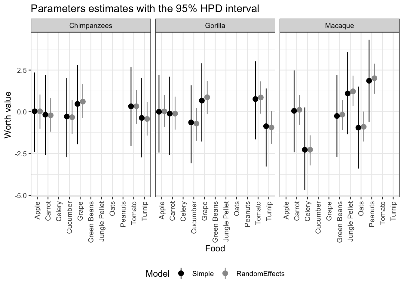

4.3.2.4 Probability of selecting a novel stimuli

We will create a the table of the predictions of selecting a novel stimuli (compared to the trained ones). This is replication of table II of the original paper (of course the results are not the same since we are using different models and estimation values)

For that, we first create a data frame of the new predictions for each species. Since our model uses random effects and we would need to specify each random effect to make the predictions we will do something slightly different. We will consider that the random effects will be zero, that is, which is equivalent to the average value of the random effects (remember that it has a mean of zero). One way to achieve this is by using the obtained coefficients in a submodel. This can be done in the bpcs package by using the model_type option.

We ask for the data frame instead of the table because we will assemble the table manually.

# Create a data frame with all the pairs of food that we want to calculate
pairs_gor <-
  data.frame(
    image2 = c(
      'Apple',
      'Apple',
      'Apple',
      'Apple',
      'Tomato',
      'Tomato',
      'Tomato',
      'Tomato'
    ),
    image1 = c(
      'Cucumber',
      'Grape',
      'Turnip',
      'Carrot',
      'Cucumber',
      'Grape',
      'Turnip',
      'Carrot'
    )
  )

pairs_chip <-
  data.frame(
    image2 = c(
      'Apple',
      'Apple',
      'Apple',
      'Apple',
      'Tomato',
      'Tomato',
      'Tomato',
      'Tomato'
    ),
    image1 = c(
      'Cucumber',
      'Grape',
      'Turnip',
      'Carrot',
      'Cucumber',
      'Grape',
      'Turnip',
      'Carrot'
    )
  )


pairs_macaque <-
  data.frame(
    image2 = c(
      'Oats',
      'Oats',
      'Oats',
      'Oats',
      'Green Beans',
      'Green Beans',
      'Green Beans',
      'Green Beans'
    ),
    image1 = c(
      'Celery',
      'Jungle Pellet',
      'Peanuts',
      'Carrot',
      'Celery',
      'Jungle Pellet',
      'Peanuts',
      'Carrot'
    )
  )


prob_chip <-
  get_probabilities_df(
    m2_chip, 
    newdata = pairs_chip,
    model_type = 'bt')

prob_macaque <-
  get_probabilities_df(
    m2_macaque, 
    newdata = pairs_macaque, 
    model_type = 'bt')

prob_gor <-
  get_probabilities_df(
    m2_gor, 
    newdata = pairs_gor, 
    model_type = 'bt')

#merging in a single df
prob_table <- rbind(prob_gor, prob_chip, prob_macaque)

Now we can create the table

prob_table <- prob_table %>%
  mutate(Probability = i_beats_j,
         OddsRatio = Probability / (1 - Probability))

prob_table %>%
  dplyr::select(i, j, Probability, OddsRatio) %>%
  kable(
    caption = 'Posterior probabilities of the novel stimuli i being selected over the trained stimuli j',
    booktabs = T,
    digits = 2,
    col.names = c('Item i', 'Item j', 'Probability', 'Odds Ratio')
  ) %>%
  kableExtra::kable_styling(bootstrap_options = c("striped", "hover", "condensed", "responsive")) %>%
  kableExtra::pack_rows("Gorilla", 1, 8) %>%
  kableExtra::pack_rows("Chimpanzee", 9, 16) %>%
  kableExtra::pack_rows("Macaque", 17, 24) %>% 
  kableExtra::scroll_box(width = "100%")

Table 4.8: Posterior probabilities of the novel stimuli i being selected over the trained stimuli j
Item i	Item j	Probability	Odds Ratio
Gorilla
Apple	Cucumber	0.63	1.70
Apple	Grape	0.29	0.41
Apple	Turnip	0.77	3.35
Apple	Carrot	0.56	1.27
Tomato	Cucumber	0.84	5.25
Tomato	Grape	0.50	1.00
Tomato	Turnip	0.87	6.69
Tomato	Carrot	0.70	2.33
Chimpanzee
Apple	Cucumber	0.56	1.27
Apple	Grape	0.31	0.45
Apple	Turnip	0.61	1.56
Apple	Carrot	0.53	1.13
Tomato	Cucumber	0.64	1.78
Tomato	Grape	0.39	0.64
Tomato	Turnip	0.73	2.70
Tomato	Carrot	0.52	1.08
Macaque
Oats	Celery	0.73	2.70
Oats	Jungle Pellet	0.08	0.09
Oats	Peanuts	0.01	0.01
Oats	Carrot	0.25	0.33
Green Beans	Celery	0.93	13.29
Green Beans	Jungle Pellet	0.22	0.28
Green Beans	Peanuts	0.17	0.20
Green Beans	Carrot	0.49	0.96