Random effects in the Bradley-Terry model
Source:vignettes/c_bt_random_effects.Rmd
c_bt_random_effects.RmdIntroduction
In this vignette, we will go over an example of analyzing optimization algorithms based on benchmark functions. A extended analysis of this example including the experimental conditions for the data collection is discussed in “Statistical Models for the Analysis of Optimization Algorithms with Benchmark Functions”
In the development of optimization algorithms it is common to use benchmark functions/problems to show:
- The algorithm works on a number of the artificial problems
- Compare how different algorithms perform in the same set of benchmark problems that have a known solution.
In the comparison part, researchers usually select a small number of benchmark problems (something like 20-30) and run their algorithms and the algorithms they are comparing several times for the same benchmark (something like 10 times each algorithm in each benchmark). At the end, they compare how close the algorithms approached the solution and rank them.
Almost always, this comparison is done with non-parametric tests statistics and often fail to compute the intra-class correlation of the repeated-measures, or average the repeated measures (throwing out the uncertainty of the results) before running the tests.
Why use ranks and not the output directly?
Each benchmark function has a different search space and the algorithms converge quite differently from one function to the other. While the difference between the minimum and the algorithm output is limited to zero (when they solve the problem), the difference can range from 0.1 to 100 depending on the benchmark problem. To use this value would require either transformations such as normalizing for each benchmark. However, if we want only to rank the algorithms and provide a classification between them, the Bradley-Terry model is ideal. The differences in range of each benchmark function is already taken care of when computing who wins and who looses.
In this example, we will show how to use the Bradley-Terry model to compensate the dependent data of the repeated measures and rank the algorithms. Our Bradley-Terry ranking of the abilities also shows the uncertainty of the ranks and the probabilities of one algorithm beating the other in any of the benchmarks.
The data
First let’s load some packages
library(bpcs)
library(dplyr)
library(tidyr)
library(ggplot2)
library(kableExtra)
library(knitr)
library(gtools)
library(bayesplot)
The collected data is available as:
data("optimization_algorithms")
knitr::kable(dplyr::sample_n(optimization_algorithms, size = 20),
caption = "Sample of the data set")| Algorithm | Benchmark | TrueRewardDifference | Ndimensions | MaxFevalPerDimensions | simNumber |
|---|---|---|---|---|---|
| SimulatedAnnealing | DiscusN2 | 1.658642e-01 | 2 | 1e+05 | 4 |
| SimulatedAnnealing | Schwefel2d20N2 | 4.914597e+01 | 2 | 1e+05 | 8 |
| RandomSearch1 | Trigonometric1N6 | 0.000000e+00 | 6 | 1e+05 | 7 |
| PSO | Schwefel2d20N2 | 8.100000e-04 | 2 | 1e+05 | 3 |
| DifferentialEvolution | ChenV | 0.000000e+00 | 2 | 1e+05 | 1 |
| NelderMead | Damavandi | 3.261795e+00 | 2 | 1e+05 | 0 |
| DifferentialEvolution | ChenBird | 1.000004e+03 | 2 | 1e+05 | 9 |
| NelderMead | Damavandi | 4.283515e+01 | 2 | 1e+05 | 6 |
| PSO | Schwefel2d4N6 | 1.708593e+00 | 6 | 1e+05 | 7 |
| NelderMead | LunacekBiRastriginN6 | 1.111721e+02 | 6 | 1e+05 | 7 |
| SimulatedAnnealing | PinterN6 | 1.089849e+02 | 6 | 1e+05 | 1 |
| SimulatedAnnealing | Giunta | 4.000000e-07 | 2 | 1e+05 | 8 |
| SimulatedAnnealing | Schwefel2d20N2 | 4.461370e-02 | 2 | 1e+05 | 1 |
| NelderMead | QingN2 | 1.855444e+07 | 2 | 1e+05 | 4 |
| NelderMead | SalomonN2 | 4.333972e+00 | 2 | 1e+05 | 5 |
| NelderMead | Damavandi | 4.328056e+00 | 2 | 1e+05 | 4 |
| DifferentialEvolution | SphereN6 | 0.000000e+00 | 6 | 1e+05 | 1 |
| RandomSearch1 | Tripod | 1.706088e-01 | 2 | 1e+05 | 1 |
| PSO | ChenV | 1.000028e+03 | 2 | 1e+05 | 5 |
| PSO | Tripod | 1.001476e+00 | 2 | 1e+05 | 4 |
In this dataset, we have one main metrics that we can use to compare the algorithms. The TrueRewardDifference is the difference between the minimum found by the algorithm and the global minimum of the benchmark function. simNumber indicates the number of the replication of the same algorithm in the same benchmark function (but with different seeds). All algorithms had a budget of 10,000 function evaluations per number of dimensions for each benchmark function.
Here we have the following benchmark functions:
bm <- unique(optimization_algorithms$Benchmark)
nbm <- length(bm)
knitr::kable(matrix(bm, ncol = 4))
#> Warning in matrix(bm, ncol = 4): data length [30] is not a sub-multiple or
#> multiple of the number of rows [8]| BentCigarN6 | LunacekBiRastriginN6 | Schwefel2d21N6 | Trefethen |
| ChenBird | Mishra7N6 | Schwefel2d23N6 | Trigonometric1N6 |
| ChenV | PinterN6 | Schwefel2d26N6 | Tripod |
| ChungReynoldsN2 | Price1 | Schwefel2d4N6 | WhitleyN6 |
| Damavandi | QingN2 | Shubert | XinSheYang2N2 |
| DiscusN2 | RosenbrockRotatedN6 | SphereN6 | ZakharovN2 |
| ExponentialN2 | SalomonN2 | StrechedVSineWave2N | BentCigarN6 |
| Giunta | Schwefel2d20N2 | ThreeHumpCamelBack | ChenBird |
To reduce a bit the model sampling time here lets reduce the number of benchmark functions and only use 10 of them.
set.seed(1)
bm_reduced <- sample(size = 10, x = bm, replace = F)
optimization_algorithms <- optimization_algorithms %>%
  dplyr::filter(Benchmark %in% bm_reduced)
knitr::kable(matrix(bm_reduced, ncol = 2))| Trefethen | StrechedVSineWave2N |
| ChungReynoldsN2 | PinterN6 |
| ExponentialN2 | RosenbrockRotatedN6 |
| BentCigarN6 | Schwefel2d23N6 |
| ChenBird | Schwefel2d26N6 |
Here we have the optimization algorithms:
| x |
|---|
| NelderMead |
| PSO |
| SimulatedAnnealing |
| DifferentialEvolution |
| RandomSearch1 |
| CMAES |
Preparing the data
To analyze this data we first need to convert it to a paired comparison. We will do it in the following way:
- First we group and rank the algorithms for each benchmark function in each simNumber. If there are ties (not very likely in this case) we will solve them randomly
- We expand this dataset into a wide format in the ranks. Each new column will contain the rank of the algorithms
- We expand this wide format to a long format with each of the paired comparisons.
To compute all the paired combinations between the algorithms we will use the gtools::comb function
comb <- gtools::combinations(n=nalg, r=2, v=seq(1:nalg), repeats.allowed = F)Creating the dataset
#1 Grouping and ranking
df_1 <-
  optimization_algorithms %>%  dplyr::group_by(Benchmark, simNumber) %>%
  dplyr::mutate(rankReward = rank(TrueRewardDifference, ties.method = 'random')) %>%
  dplyr::ungroup() %>%
  dplyr::select(-TrueRewardDifference)

#2 Expanding in wide format
df_2 <- df_1 %>%
  tidyr::pivot_wider(names_from = Algorithm,
                     values_from = rankReward) %>%
  dplyr::select(-MaxFevalPerDimensions,-Ndimensions) #dropping some variables that we will not use

#3 Computing the paired comparisons
## Maybe not the most efficient code, but for this number of variables it is fast enough, only a few seconds...
#We first go row by row of the wide data frame df_2 and expand each row into the number of combinations
#available of the different ranks
df_3 <-
  dplyr::tribble( ~ algo0_name, ~ algo1_name, ~ y, ~ simNumber, ~ Benchmark)

for (i in 1:nrow(df_2))
{
  current_row <- df_2[i, ]
  for (j in 1:nrow(comb)) {
    comb_row <- comb[j, ]

    algo0_name <- alg[comb_row[1]]
    algo0 <- comb_row[1]
    algo0_rank <- current_row[[1, algo0_name]]

    algo1_name <- alg[comb_row[2]]
    algo1 <- comb_row[2]
    algo1_rank <- current_row[[1, algo1_name]]

    diff_rank <- algo1_rank - algo0_rank
    y <-
      ifelse(diff_rank < 0, 1, 0) # if rank0 is higher than rank1, algo1 wins
    df_3 <- tibble::add_row(
      df_3,
      algo0_name = algo0_name,
      algo1_name = algo1_name,
      y = y,
      simNumber = current_row$simNumber,
      Benchmark = current_row$Benchmark
    )
  }
}
df_3 <- as.data.frame(df_3)
The table below shows how the dataset looks like now.
dplyr::sample_n(df_3,size = 20)
#>               algo0_name            algo1_name y simNumber           Benchmark
#> 1  DifferentialEvolution                 CMAES 1         7         BentCigarN6
#> 2          RandomSearch1                 CMAES 1         2       ExponentialN2
#> 3             NelderMead         RandomSearch1 1         7         BentCigarN6
#> 4                    PSO                 CMAES 1         4       ExponentialN2
#> 5  DifferentialEvolution                 CMAES 1         5       ExponentialN2
#> 6             NelderMead DifferentialEvolution 1         0 RosenbrockRotatedN6
#> 7             NelderMead                   PSO 1         4 RosenbrockRotatedN6
#> 8             NelderMead DifferentialEvolution 1         6     ChungReynoldsN2
#> 9             NelderMead DifferentialEvolution 1         3            PinterN6
#> 10         RandomSearch1                 CMAES 0         3      Schwefel2d26N6
#> 11         RandomSearch1                 CMAES 1         2         BentCigarN6
#> 12            NelderMead    SimulatedAnnealing 0         0      Schwefel2d23N6
#> 13                   PSO DifferentialEvolution 1         7         BentCigarN6
#> 14            NelderMead                   PSO 1         0      Schwefel2d26N6
#> 15    SimulatedAnnealing DifferentialEvolution 1         2      Schwefel2d23N6
#> 16    SimulatedAnnealing                 CMAES 1         4            ChenBird
#> 17    SimulatedAnnealing         RandomSearch1 1         7            ChenBird
#> 18                   PSO         RandomSearch1 0         0            ChenBird
#> 19                   PSO                 CMAES 1         8         BentCigarN6
#> 20                   PSO                 CMAES 1         1 RosenbrockRotatedN6
The model
To compensate for the repeated measures model we will use the random effects model. The model can be written as:
For the benchmark \(k\) we have: \[P[i \text{ beats } j | U_k]= \dfrac{exp(\lambda_i + U_{i,k})}{exp(\lambda_i + U_{i,k}) + exp(\lambda_j + U_{j,k})}\]
\[\lambda \sim \text{Normal}(0,3.0)\] \[U \sim \text{Normal}(0,3.0)\]
Now we can estimate and control the effect of each benchmark in each algorithm when we estimate the ability parameter. This model will estimate the parameters \(\lambda\) and \(U\) of the model. Note that the model with many parameters and data points might take a few minutes to sample.
Lets also specify a wide prior for the standard deviation of the random effects. This will help the convergence
m <-
  bpc(
    data = df_3,
    player0 = 'algo0_name',
    player1 = 'algo1_name',
    result_column = 'y',
    cluster = 'Benchmark',
    model_type = 'bt-U',
    priors = list(prior_U1_std = 10.0)
  )
#> Running MCMC with 4 parallel chains...
#>
#> Chain 3 finished in 447.0 seconds.
#> Chain 4 finished in 449.4 seconds.
#> Chain 1 finished in 453.5 seconds.
#> Chain 2 finished in 464.1 seconds.
#>
#> All 4 chains finished successfully.
#> Mean chain execution time: 453.5 seconds.
#> Total execution time: 464.4 seconds.
Diagnostics
First let’s look at the MCMC convergence with the traceplots and look at the Rhat and neff
get_parameters_df(m, n_eff = T, Rhat = T)
#>                                        Parameter        Mean      Median
#> 1                             lambda[NelderMead] -6.10810972 -6.12350500
#> 2                                    lambda[PSO]  1.90441804  1.89784500
#> 3                     lambda[SimulatedAnnealing] -3.55592226 -3.55070500
#> 4                  lambda[DifferentialEvolution]  6.32010385  6.30835000
#> 5                          lambda[RandomSearch1] -1.06321251 -1.08614000
#> 6                                  lambda[CMAES]  2.60299353  2.57542000
#> 7                     U1[NelderMead,BentCigarN6] -1.00758874 -0.98139350
#> 8                            U1[PSO,BentCigarN6] -0.07753904 -0.08200790
#> 9             U1[SimulatedAnnealing,BentCigarN6] -0.27600814 -0.27076950
#> 10         U1[DifferentialEvolution,BentCigarN6] -0.27008696 -0.26894600
#> 11                 U1[RandomSearch1,BentCigarN6] -0.37172490 -0.36906700
#> 12                         U1[CMAES,BentCigarN6]  1.98923669  1.97657000
#> 13                       U1[NelderMead,ChenBird]  0.15165166  0.15543150
#> 14                              U1[PSO,ChenBird] -0.18351594 -0.19157850
#> 15               U1[SimulatedAnnealing,ChenBird] -0.94637713 -0.94557550
#> 16            U1[DifferentialEvolution,ChenBird] -0.33725296 -0.34428800
#> 17                    U1[RandomSearch1,ChenBird] -0.55481582 -0.55026600
#> 18                            U1[CMAES,ChenBird]  1.93082862  1.91112000
#> 19                U1[NelderMead,ChungReynoldsN2] -0.31749361 -0.30858850
#> 20                       U1[PSO,ChungReynoldsN2]  0.07453414  0.06466390
#> 21        U1[SimulatedAnnealing,ChungReynoldsN2] -0.96540562 -0.96101050
#> 22     U1[DifferentialEvolution,ChungReynoldsN2]  0.94343669  0.91907050
#> 23             U1[RandomSearch1,ChungReynoldsN2] -0.25571713 -0.24913200
#> 24                     U1[CMAES,ChungReynoldsN2]  0.52904367  0.53480150
#> 25                  U1[NelderMead,ExponentialN2] -0.66141727 -0.62704750
#> 26                         U1[PSO,ExponentialN2] -0.04723910 -0.04996835
#> 27          U1[SimulatedAnnealing,ExponentialN2]  0.38188001  0.37733900
#> 28       U1[DifferentialEvolution,ExponentialN2] -0.39059440 -0.38545950
#> 29               U1[RandomSearch1,ExponentialN2] -0.05669672 -0.05196185
#> 30                       U1[CMAES,ExponentialN2]  0.80567842  0.79661900
#> 31                       U1[NelderMead,PinterN6]  0.15593465  0.16700100
#> 32                              U1[PSO,PinterN6]  0.08552279  0.08313760
#> 33               U1[SimulatedAnnealing,PinterN6]  0.52786695  0.52568350
#> 34            U1[DifferentialEvolution,PinterN6]  0.58833364  0.54973600
#> 35                    U1[RandomSearch1,PinterN6]  0.06078388  0.06025335
#> 36                            U1[CMAES,PinterN6] -1.40808557 -1.40093500
#> 37            U1[NelderMead,RosenbrockRotatedN6] -0.37853226 -0.36856000
#> 38                   U1[PSO,RosenbrockRotatedN6]  0.17055384  0.16737150
#> 39    U1[SimulatedAnnealing,RosenbrockRotatedN6] -0.35664793 -0.34720250
#> 40 U1[DifferentialEvolution,RosenbrockRotatedN6]  0.13451722  0.13433350
#> 41         U1[RandomSearch1,RosenbrockRotatedN6] -0.35692088 -0.34738750
#> 42                 U1[CMAES,RosenbrockRotatedN6]  0.75279310  0.74384000
#> 43                 U1[NelderMead,Schwefel2d23N6] -0.11225531 -0.11109950
#> 44                        U1[PSO,Schwefel2d23N6] -0.10121956 -0.09974590
#> 45         U1[SimulatedAnnealing,Schwefel2d23N6] -1.33004846 -1.32729000
#> 46      U1[DifferentialEvolution,Schwefel2d23N6]  1.09996531  1.07526500
#> 47              U1[RandomSearch1,Schwefel2d23N6] -0.33655185 -0.33647000
#> 48                      U1[CMAES,Schwefel2d23N6]  0.81540015  0.81484200
#> 49                 U1[NelderMead,Schwefel2d26N6]  0.77222373  0.76481850
#> 50                        U1[PSO,Schwefel2d26N6] -0.95513714 -0.95481500
#> 51         U1[SimulatedAnnealing,Schwefel2d26N6]  0.04467586  0.04283875
#> 52      U1[DifferentialEvolution,Schwefel2d26N6] -0.28249294 -0.28819600
#> 53              U1[RandomSearch1,Schwefel2d26N6]  1.05542501  1.04452000
#> 54                      U1[CMAES,Schwefel2d26N6] -0.67916286 -0.68133000
#> 55            U1[NelderMead,StrechedVSineWave2N] -0.14393381 -0.14626450
#> 56                   U1[PSO,StrechedVSineWave2N]  0.65333062  0.64341450
#> 57    U1[SimulatedAnnealing,StrechedVSineWave2N]  0.73342395  0.72676400
#> 58 U1[DifferentialEvolution,StrechedVSineWave2N]  0.87519950  0.84686800
#> 59         U1[RandomSearch1,StrechedVSineWave2N]  0.22209742  0.21388650
#> 60                 U1[CMAES,StrechedVSineWave2N] -2.33926506 -2.33498500
#> 61                      U1[NelderMead,Trefethen] -0.65145296 -0.61850000
#> 62                             U1[PSO,Trefethen]  1.11266440  1.11640000
#> 63              U1[SimulatedAnnealing,Trefethen]  0.87042565  0.86282700
#> 64           U1[DifferentialEvolution,Trefethen] -0.09594043 -0.10590850
#> 65                   U1[RandomSearch1,Trefethen]  0.25820381  0.26490650
#> 66                           U1[CMAES,Trefethen] -1.49136053 -1.48878000
#> 67                                        U1_std  3.28660341  3.21802500
#>     HPD_lower HPD_higher   Rhat n_eff
#> 1  -9.3110700 -2.9710400 1.0006  6821
#> 2  -1.1995800  4.9463900 1.0001  6455
#> 3  -6.5660400 -0.4842180 1.0002  6467
#> 4   3.1029200  9.4034400 1.0001  7157
#> 5  -4.1313800  1.9371600 1.0006  6270
#> 6  -0.4521180  5.6673800 1.0010  6794
#> 7  -2.4406900  0.3706760 0.9998  9698
#> 8  -1.2316000  1.0643300 1.0007  8403
#> 9  -1.4196600  0.8820330 1.0008  8174
#> 10 -1.5007900  0.9407810 1.0005  8974
#> 11 -1.5763800  0.7027340 1.0012  7922
#> 12  0.6749780  3.3008400 1.0000  9050
#> 13 -1.0046100  1.2793800 1.0001  7915
#> 14 -1.3693100  0.9577270 1.0004  8345
#> 15 -2.1006700  0.2139620 1.0002  7978
#> 16 -1.4966100  0.8993270 1.0001  8701
#> 17 -1.7103400  0.5362900 1.0006  7973
#> 18  0.6492880  3.2622800 1.0000  9303
#> 19 -1.5302600  0.9153230 0.9999  8745
#> 20 -1.0695700  1.1922900 0.9998  8324
#> 21 -2.1377200  0.2630240 1.0000  8380
#> 22 -0.4556840  2.3838600 1.0007  9767
#> 23 -1.3998800  0.8974950 1.0002  7848
#> 24 -0.6018150  1.6984700 1.0003  8397
#> 25 -2.1350000  0.8019950 1.0003  9818
#> 26 -1.0848800  1.0374300 1.0005  6910
#> 27 -0.7307690  1.4534500 0.9999  7138
#> 28 -1.4874800  0.7690870 1.0003  7998
#> 29 -1.0818400  1.0632800 1.0008  6927
#> 30 -0.3434110  1.8840400 1.0005  7746
#> 31 -0.9723120  1.3357100 1.0004  7496
#> 32 -0.9915230  1.1837200 0.9998  7210
#> 33 -0.5495750  1.5805300 1.0008  6808
#> 34 -0.8542200  2.1618000 1.0002 11777
#> 35 -0.9667000  1.1104400 0.9998  6833
#> 36 -2.5371500 -0.3323380 1.0004  5944
#> 37 -1.5962600  0.8530750 1.0005  7939
#> 38 -1.0129400  1.2802500 0.9999  7668
#> 39 -1.5021300  0.7532060 1.0002  7631
#> 40 -1.0220400  1.3057600 0.9998  8557
#> 41 -1.4560400  0.7753630 1.0005  7036
#> 42 -0.3904240  1.9401000 1.0000  7905
#> 43 -1.3007800  1.1277800 0.9999  8330
#> 44 -1.2230900  1.0699600 1.0006  8411
#> 45 -2.5077200 -0.0853162 0.9997  8346
#> 46 -0.3225130  2.4944800 0.9998  9806
#> 47 -1.5008000  0.8008400 1.0004  7905
#> 48 -0.3759100  2.0022300 1.0003  8905
#> 49 -0.3082910  1.8328800 1.0000  6991
#> 50 -1.9576800  0.1559700 1.0010  6673
#> 51 -1.0236600  1.0608600 1.0000  7059
#> 52 -1.4883700  0.8827520 1.0001  8229
#> 53  0.0290641  2.1566500 1.0005  5992
#> 54 -1.7180500  0.3363720 1.0008  7041
#> 55 -1.3240200  0.9932460 1.0000  7570
#> 56 -0.5481430  1.8615400 0.9997  9000
#> 57 -0.3426310  1.8987600 1.0004  7054
#> 58 -0.5639240  2.2952400 1.0003  9014
#> 59 -0.8253850  1.3523200 0.9999  7215
#> 60 -3.5605000 -1.1143100 1.0010  6763
#> 61 -2.1487000  0.8386380 1.0003  9458
#> 62 -0.1298920  2.2861600 1.0005  8703
#> 63 -0.2439750  1.9468900 1.0010  7251
#> 64 -1.3400200  1.1089600 1.0008  9532
#> 65 -0.9087470  1.2620600 0.9998  7778
#> 66 -2.6059100 -0.3805550 1.0002  7424
#> 67  2.2476200  4.4012900 1.0004  3496
All seems ok! Let’s look now at the traceplots
Traceplots of the chains with the bayesplot library
fit <- get_fit(m)
posterior_draws <- posterior::as_draws_matrix(fit$draws())
bayesplot::mcmc_trace(
  posterior_draws,
  pars = c(
    "lambda[1]",
    "lambda[2]",
    "lambda[3]",
    "lambda[4]",
    "lambda[5]",
    "lambda[6]",
    "U1_std"
  ),
  n_warmup = 1000
)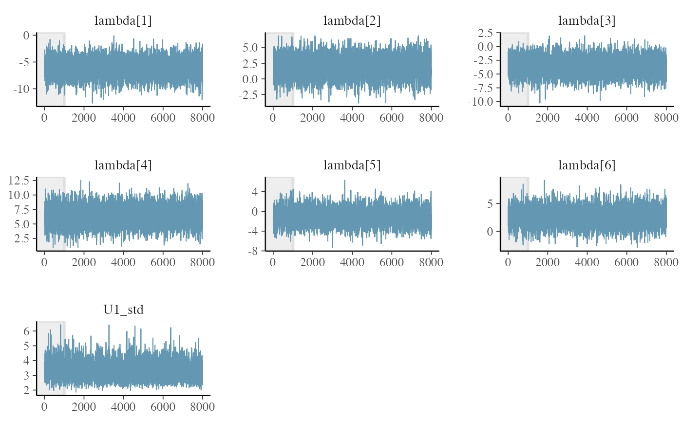
Everything seems in order for us to look at the predictive posterior bar plot.
y_pp <- posterior_predictive(m)
y <- y_pp$y
yrep <- y_pp$y_pred
bayesplot::ppc_bars(y = df_3$y, yrep = yrep) +
  labs(title = 'Bar plot with medians and uncertainty\n intervals superimposed')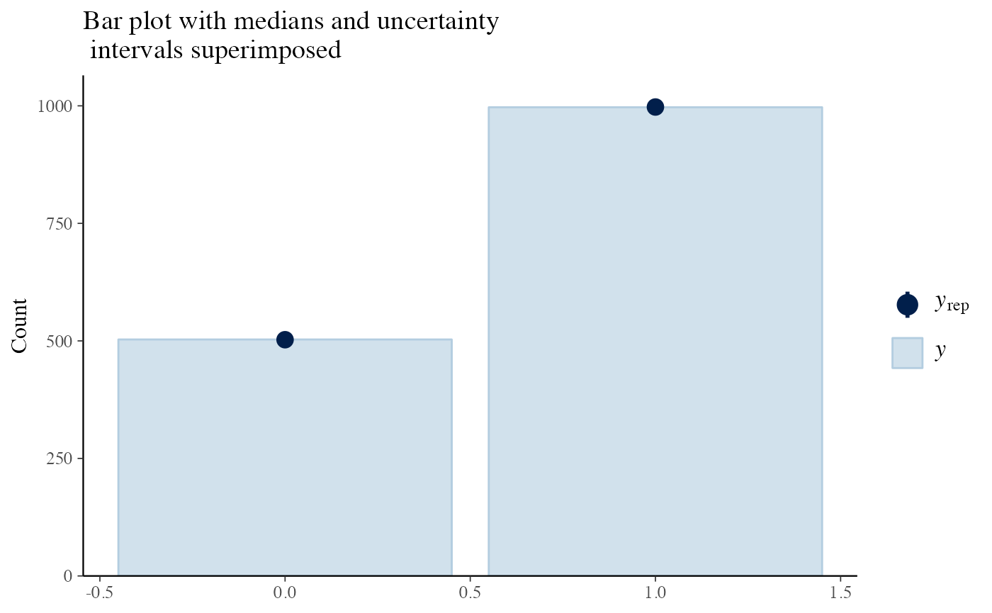
This sounds ok. So let’s investigate the actual parameters and the probabilities of the models
Summary parameters
In the console, we can use the summary function. It gives the parameters estimates with HPDI, the probability table for every condition of players and benchmarks and we also have a rank estimate.
summary(m)
#> Estimated baseline parameters with 95% HPD intervals:
#>
#> Table: Parameters estimates
#>
#> Parameter                                         Mean   Median   HPD_lower   HPD_higher
#> ----------------------------------------------  ------  -------  ----------  -----------
#> lambda[NelderMead]                               -6.11    -6.12       -9.31        -2.97
#> lambda[PSO]                                       1.90     1.90       -1.20         4.95
#> lambda[SimulatedAnnealing]                       -3.56    -3.55       -6.57        -0.48
#> lambda[DifferentialEvolution]                     6.32     6.31        3.10         9.40
#> lambda[RandomSearch1]                            -1.06    -1.09       -4.13         1.94
#> lambda[CMAES]                                     2.60     2.58       -0.45         5.67
#> U1[NelderMead,BentCigarN6]                       -1.01    -0.98       -2.44         0.37
#> U1[PSO,BentCigarN6]                              -0.08    -0.08       -1.23         1.06
#> U1[SimulatedAnnealing,BentCigarN6]               -0.28    -0.27       -1.42         0.88
#> U1[DifferentialEvolution,BentCigarN6]            -0.27    -0.27       -1.50         0.94
#> U1[RandomSearch1,BentCigarN6]                    -0.37    -0.37       -1.58         0.70
#> U1[CMAES,BentCigarN6]                             1.99     1.98        0.67         3.30
#> U1[NelderMead,ChenBird]                           0.15     0.16       -1.00         1.28
#> U1[PSO,ChenBird]                                 -0.18    -0.19       -1.37         0.96
#> U1[SimulatedAnnealing,ChenBird]                  -0.95    -0.95       -2.10         0.21
#> U1[DifferentialEvolution,ChenBird]               -0.34    -0.34       -1.50         0.90
#> U1[RandomSearch1,ChenBird]                       -0.55    -0.55       -1.71         0.54
#> U1[CMAES,ChenBird]                                1.93     1.91        0.65         3.26
#> U1[NelderMead,ChungReynoldsN2]                   -0.32    -0.31       -1.53         0.92
#> U1[PSO,ChungReynoldsN2]                           0.07     0.06       -1.07         1.19
#> U1[SimulatedAnnealing,ChungReynoldsN2]           -0.97    -0.96       -2.14         0.26
#> U1[DifferentialEvolution,ChungReynoldsN2]         0.94     0.92       -0.46         2.38
#> U1[RandomSearch1,ChungReynoldsN2]                -0.26    -0.25       -1.40         0.90
#> U1[CMAES,ChungReynoldsN2]                         0.53     0.53       -0.60         1.70
#> U1[NelderMead,ExponentialN2]                     -0.66    -0.63       -2.13         0.80
#> U1[PSO,ExponentialN2]                            -0.05    -0.05       -1.08         1.04
#> U1[SimulatedAnnealing,ExponentialN2]              0.38     0.38       -0.73         1.45
#> U1[DifferentialEvolution,ExponentialN2]          -0.39    -0.39       -1.49         0.77
#> U1[RandomSearch1,ExponentialN2]                  -0.06    -0.05       -1.08         1.06
#> U1[CMAES,ExponentialN2]                           0.81     0.80       -0.34         1.88
#> U1[NelderMead,PinterN6]                           0.16     0.17       -0.97         1.34
#> U1[PSO,PinterN6]                                  0.09     0.08       -0.99         1.18
#> U1[SimulatedAnnealing,PinterN6]                   0.53     0.53       -0.55         1.58
#> U1[DifferentialEvolution,PinterN6]                0.59     0.55       -0.85         2.16
#> U1[RandomSearch1,PinterN6]                        0.06     0.06       -0.97         1.11
#> U1[CMAES,PinterN6]                               -1.41    -1.40       -2.54        -0.33
#> U1[NelderMead,RosenbrockRotatedN6]               -0.38    -0.37       -1.60         0.85
#> U1[PSO,RosenbrockRotatedN6]                       0.17     0.17       -1.01         1.28
#> U1[SimulatedAnnealing,RosenbrockRotatedN6]       -0.36    -0.35       -1.50         0.75
#> U1[DifferentialEvolution,RosenbrockRotatedN6]     0.13     0.13       -1.02         1.31
#> U1[RandomSearch1,RosenbrockRotatedN6]            -0.36    -0.35       -1.46         0.78
#> U1[CMAES,RosenbrockRotatedN6]                     0.75     0.74       -0.39         1.94
#> U1[NelderMead,Schwefel2d23N6]                    -0.11    -0.11       -1.30         1.13
#> U1[PSO,Schwefel2d23N6]                           -0.10    -0.10       -1.22         1.07
#> U1[SimulatedAnnealing,Schwefel2d23N6]            -1.33    -1.33       -2.51        -0.09
#> U1[DifferentialEvolution,Schwefel2d23N6]          1.10     1.08       -0.32         2.49
#> U1[RandomSearch1,Schwefel2d23N6]                 -0.34    -0.34       -1.50         0.80
#> U1[CMAES,Schwefel2d23N6]                          0.82     0.81       -0.38         2.00
#> U1[NelderMead,Schwefel2d26N6]                     0.77     0.76       -0.31         1.83
#> U1[PSO,Schwefel2d26N6]                           -0.96    -0.95       -1.96         0.16
#> U1[SimulatedAnnealing,Schwefel2d26N6]             0.04     0.04       -1.02         1.06
#> U1[DifferentialEvolution,Schwefel2d26N6]         -0.28    -0.29       -1.49         0.88
#> U1[RandomSearch1,Schwefel2d26N6]                  1.06     1.04        0.03         2.16
#> U1[CMAES,Schwefel2d26N6]                         -0.68    -0.68       -1.72         0.34
#> U1[NelderMead,StrechedVSineWave2N]               -0.14    -0.15       -1.32         0.99
#> U1[PSO,StrechedVSineWave2N]                       0.65     0.64       -0.55         1.86
#> U1[SimulatedAnnealing,StrechedVSineWave2N]        0.73     0.73       -0.34         1.90
#> U1[DifferentialEvolution,StrechedVSineWave2N]     0.88     0.85       -0.56         2.30
#> U1[RandomSearch1,StrechedVSineWave2N]             0.22     0.21       -0.83         1.35
#> U1[CMAES,StrechedVSineWave2N]                    -2.34    -2.33       -3.56        -1.11
#> U1[NelderMead,Trefethen]                         -0.65    -0.62       -2.15         0.84
#> U1[PSO,Trefethen]                                 1.11     1.12       -0.13         2.29
#> U1[SimulatedAnnealing,Trefethen]                  0.87     0.86       -0.24         1.95
#> U1[DifferentialEvolution,Trefethen]              -0.10    -0.11       -1.34         1.11
#> U1[RandomSearch1,Trefethen]                       0.26     0.26       -0.91         1.26
#> U1[CMAES,Trefethen]                              -1.49    -1.49       -2.61        -0.38
#> U1_std                                            3.29     3.22        2.25         4.40
#> NOTES:
#> * A higher lambda indicates a higher team ability
#> * The U_std indicates the standard deviation of the normal distribution where the parameters U[player, cluster] are drawn from. Higher values of U_std indicates a higher effect of the cluster in the team abitilies.
#> * The U[player, cluster] represents the effect of a particular cluster in a particular team ability.
#>
#> Rank of the players' abilities:
#> The rank is based on the posterior rank distribution of the lambda parameter
#>
#> Table: Estimated posterior ranks
#>
#> Parameter                MedianRank   MeanRank   StdRank
#> ----------------------  -----------  ---------  --------
#> DifferentialEvolution             1       1.01      0.09
#> CMAES                             2       2.33      0.49
#> PSO                               3       2.68      0.51
#> RandomSearch1                     4       4.03      0.27
#> SimulatedAnnealing                5       5.00      0.30
#> NelderMead                        6       5.96      0.21
Of course we can get these estimates in nicer tables with kable that allows a greater deal of customization
get_parameters_table(m, format = 'html')| Parameter | Mean | Median | HPD_lower | HPD_higher |
|---|---|---|---|---|
| lambda[NelderMead] | -6.108 | -6.124 | -9.311 | -2.971 |
| lambda[PSO] | 1.904 | 1.898 | -1.200 | 4.946 |
| lambda[SimulatedAnnealing] | -3.556 | -3.551 | -6.566 | -0.484 |
| lambda[DifferentialEvolution] | 6.320 | 6.308 | 3.103 | 9.403 |
| lambda[RandomSearch1] | -1.063 | -1.086 | -4.131 | 1.937 |
| lambda[CMAES] | 2.603 | 2.575 | -0.452 | 5.667 |
| U1[NelderMead,BentCigarN6] | -1.008 | -0.981 | -2.441 | 0.371 |
| U1[PSO,BentCigarN6] | -0.078 | -0.082 | -1.232 | 1.064 |
| U1[SimulatedAnnealing,BentCigarN6] | -0.276 | -0.271 | -1.420 | 0.882 |
| U1[DifferentialEvolution,BentCigarN6] | -0.270 | -0.269 | -1.501 | 0.941 |
| U1[RandomSearch1,BentCigarN6] | -0.372 | -0.369 | -1.576 | 0.703 |
| U1[CMAES,BentCigarN6] | 1.989 | 1.977 | 0.675 | 3.301 |
| U1[NelderMead,ChenBird] | 0.152 | 0.155 | -1.005 | 1.279 |
| U1[PSO,ChenBird] | -0.184 | -0.192 | -1.369 | 0.958 |
| U1[SimulatedAnnealing,ChenBird] | -0.946 | -0.946 | -2.101 | 0.214 |
| U1[DifferentialEvolution,ChenBird] | -0.337 | -0.344 | -1.497 | 0.899 |
| U1[RandomSearch1,ChenBird] | -0.555 | -0.550 | -1.710 | 0.536 |
| U1[CMAES,ChenBird] | 1.931 | 1.911 | 0.649 | 3.262 |
| U1[NelderMead,ChungReynoldsN2] | -0.317 | -0.309 | -1.530 | 0.915 |
| U1[PSO,ChungReynoldsN2] | 0.075 | 0.065 | -1.070 | 1.192 |
| U1[SimulatedAnnealing,ChungReynoldsN2] | -0.965 | -0.961 | -2.138 | 0.263 |
| U1[DifferentialEvolution,ChungReynoldsN2] | 0.943 | 0.919 | -0.456 | 2.384 |
| U1[RandomSearch1,ChungReynoldsN2] | -0.256 | -0.249 | -1.400 | 0.897 |
| U1[CMAES,ChungReynoldsN2] | 0.529 | 0.535 | -0.602 | 1.698 |
| U1[NelderMead,ExponentialN2] | -0.661 | -0.627 | -2.135 | 0.802 |
| U1[PSO,ExponentialN2] | -0.047 | -0.050 | -1.085 | 1.037 |
| U1[SimulatedAnnealing,ExponentialN2] | 0.382 | 0.377 | -0.731 | 1.453 |
| U1[DifferentialEvolution,ExponentialN2] | -0.391 | -0.385 | -1.487 | 0.769 |
| U1[RandomSearch1,ExponentialN2] | -0.057 | -0.052 | -1.082 | 1.063 |
| U1[CMAES,ExponentialN2] | 0.806 | 0.797 | -0.343 | 1.884 |
| U1[NelderMead,PinterN6] | 0.156 | 0.167 | -0.972 | 1.336 |
| U1[PSO,PinterN6] | 0.086 | 0.083 | -0.992 | 1.184 |
| U1[SimulatedAnnealing,PinterN6] | 0.528 | 0.526 | -0.550 | 1.581 |
| U1[DifferentialEvolution,PinterN6] | 0.588 | 0.550 | -0.854 | 2.162 |
| U1[RandomSearch1,PinterN6] | 0.061 | 0.060 | -0.967 | 1.110 |
| U1[CMAES,PinterN6] | -1.408 | -1.401 | -2.537 | -0.332 |
| U1[NelderMead,RosenbrockRotatedN6] | -0.379 | -0.369 | -1.596 | 0.853 |
| U1[PSO,RosenbrockRotatedN6] | 0.171 | 0.167 | -1.013 | 1.280 |
| U1[SimulatedAnnealing,RosenbrockRotatedN6] | -0.357 | -0.347 | -1.502 | 0.753 |
| U1[DifferentialEvolution,RosenbrockRotatedN6] | 0.135 | 0.134 | -1.022 | 1.306 |
| U1[RandomSearch1,RosenbrockRotatedN6] | -0.357 | -0.347 | -1.456 | 0.775 |
| U1[CMAES,RosenbrockRotatedN6] | 0.753 | 0.744 | -0.390 | 1.940 |
| U1[NelderMead,Schwefel2d23N6] | -0.112 | -0.111 | -1.301 | 1.128 |
| U1[PSO,Schwefel2d23N6] | -0.101 | -0.100 | -1.223 | 1.070 |
| U1[SimulatedAnnealing,Schwefel2d23N6] | -1.330 | -1.327 | -2.508 | -0.085 |
| U1[DifferentialEvolution,Schwefel2d23N6] | 1.100 | 1.075 | -0.323 | 2.494 |
| U1[RandomSearch1,Schwefel2d23N6] | -0.337 | -0.336 | -1.501 | 0.801 |
| U1[CMAES,Schwefel2d23N6] | 0.815 | 0.815 | -0.376 | 2.002 |
| U1[NelderMead,Schwefel2d26N6] | 0.772 | 0.765 | -0.308 | 1.833 |
| U1[PSO,Schwefel2d26N6] | -0.955 | -0.955 | -1.958 | 0.156 |
| U1[SimulatedAnnealing,Schwefel2d26N6] | 0.045 | 0.043 | -1.024 | 1.061 |
| U1[DifferentialEvolution,Schwefel2d26N6] | -0.282 | -0.288 | -1.488 | 0.883 |
| U1[RandomSearch1,Schwefel2d26N6] | 1.055 | 1.045 | 0.029 | 2.157 |
| U1[CMAES,Schwefel2d26N6] | -0.679 | -0.681 | -1.718 | 0.336 |
| U1[NelderMead,StrechedVSineWave2N] | -0.144 | -0.146 | -1.324 | 0.993 |
| U1[PSO,StrechedVSineWave2N] | 0.653 | 0.643 | -0.548 | 1.862 |
| U1[SimulatedAnnealing,StrechedVSineWave2N] | 0.733 | 0.727 | -0.343 | 1.899 |
| U1[DifferentialEvolution,StrechedVSineWave2N] | 0.875 | 0.847 | -0.564 | 2.295 |
| U1[RandomSearch1,StrechedVSineWave2N] | 0.222 | 0.214 | -0.825 | 1.352 |
| U1[CMAES,StrechedVSineWave2N] | -2.339 | -2.335 | -3.561 | -1.114 |
| U1[NelderMead,Trefethen] | -0.651 | -0.619 | -2.149 | 0.839 |
| U1[PSO,Trefethen] | 1.113 | 1.116 | -0.130 | 2.286 |
| U1[SimulatedAnnealing,Trefethen] | 0.870 | 0.863 | -0.244 | 1.947 |
| U1[DifferentialEvolution,Trefethen] | -0.096 | -0.106 | -1.340 | 1.109 |
| U1[RandomSearch1,Trefethen] | 0.258 | 0.265 | -0.909 | 1.262 |
| U1[CMAES,Trefethen] | -1.491 | -1.489 | -2.606 | -0.381 |
| U1_std | 3.287 | 3.218 | 2.248 | 4.401 |
get_rank_of_players_table(m, format='html')| Parameter | MedianRank | MeanRank | StdRank |
|---|---|---|---|
| DifferentialEvolution | 1 | 1.010 | 0.109 |
| CMAES | 2 | 2.294 | 0.473 |
| PSO | 3 | 2.732 | 0.510 |
| RandomSearch1 | 4 | 4.010 | 0.303 |
| SimulatedAnnealing | 5 | 4.998 | 0.300 |
| NelderMead | 6 | 5.956 | 0.205 |
Plot the HPD intervals
plot(m,rotate_x_labels = T)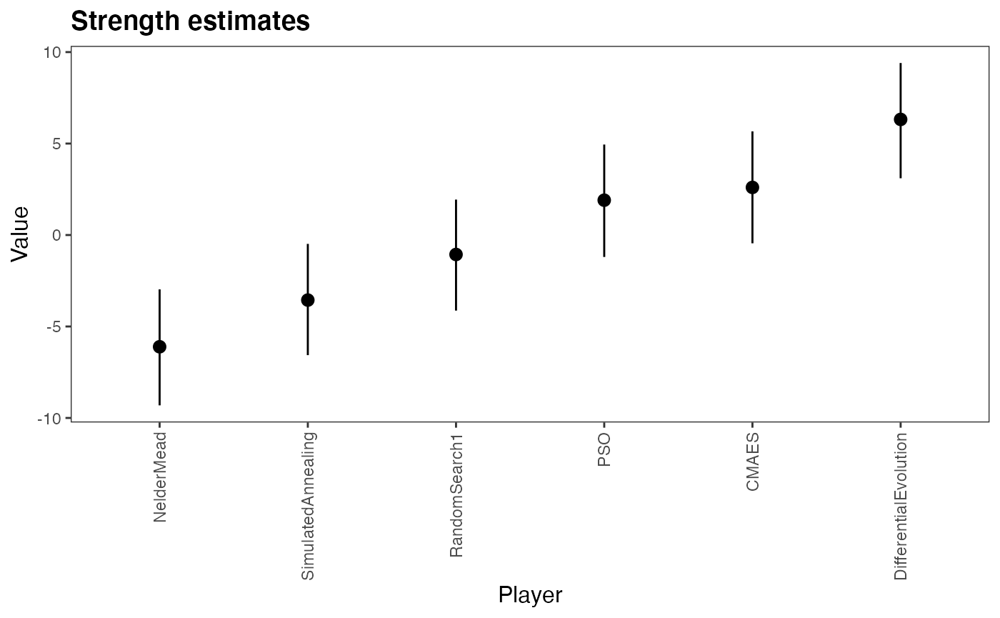
We can see that the Differential Evolution Performs better than the others. While the PSO and the CMA-ES algorithm have relatively similar abilities.
From the high value of the \(U1_{std}\) we can see that the choice of benchmarks greatly have a large variance and a big influence in the results and that some algorithms have a better performance in some benchmarks than others. E.g. the Trefethen function is a difficult problem to solve and the U estimate there seems to reduce the ability of the best algorithms while increasing the ability of the worst ones, acting as a regularizing parameter there.