library(bpcs)
library(knitr)
library(dplyr)
library(ggplot2)
library(kableExtra)

Introduction

In this vignette, we will go over a sport dataset that consists of the games from the main Brazilian football league from 2017-2019. In this example, we will create a ranking system for the teams based on the Bradley-Terry model. Then we will expand this to include ties, home-advantage effects and ties with home-advantage. Note that in this example we give equal weights to a game regardless of the date, i.e. more recent games have the same impact as older games.

The data can be accessed by:

data("brasil_soccer_league")
knitr::kable(head(brasil_soccer_league))

Time	WeekDay	Date	HomeTeam	VisitorTeam	Round	Stadium	ScoreHomeTeam	ScoreVisitorTeam
16:00	Saturday	2017-05-13	Flamengo	Atlético-MG	1	Maracanã	1	1
19:00	Saturday	2017-05-13	Corinthians	Chapecoense	1	Arena Corinthians	1	1
16:00	Sunday	2017-05-14	Avaí	Vitória	1	Ressacada	0	0
16:00	Sunday	2017-05-14	Bahia	Athlético-PR	1	Fonte Nova	6	2
16:00	Sunday	2017-05-14	Cruzeiro	São Paulo	1	Mineirão	1	0
11:00	Sunday	2017-05-14	Fluminense	Santos	1	Maracanã	3	2

Let’s analyze only the data from 2019 and remove a few columns that are not relevant for this example:

d <- brasil_soccer_league %>%
  dplyr::filter(Date >= as.Date("2019-01-01") &
                  Date <= as.Date("2019-12-31")) %>%
  dplyr::select(HomeTeam, VisitorTeam, ScoreHomeTeam, ScoreVisitorTeam, Round)

Now we have a smaller dataset (380 rows with 5 variables)

knitr::kable(head(d))

HomeTeam	VisitorTeam	ScoreHomeTeam	ScoreVisitorTeam	Round
Atlético-MG	Avaí	2	1	1
Chapecoense	Internacional	2	0	1
Flamengo	Cruzeiro	3	1	1
São Paulo	Botafogo-rj	2	0	1
Athlético-PR	Vasco	4	1	1
Bahia	Corinthians	3	2	1

Fitting a Bradley-Terry model

Let’s start fitting a simple Bradley-Terry model and handle ties randomly

m1 <- bpc(
  d,
  player0 = 'VisitorTeam',
  player1 =  'HomeTeam',
  player0_score = 'ScoreVisitorTeam',
  player1_score = 'ScoreHomeTeam',
  model_type = 'bt',
  solve_ties = 'random',
  priors = list(prior_lambda_std = 2.0),
  # making a more informative prior to improve convergence
  iter = 3000
) #stan indicates a low bulk ESS so we are increasing the number of iterations
#> Running MCMC with 4 parallel chains...
#> 
#> Chain 3 finished in 29.7 seconds.
#> Chain 1 finished in 30.2 seconds.
#> Chain 2 finished in 30.2 seconds.
#> Chain 4 finished in 30.2 seconds.
#> 
#> All 4 chains finished successfully.
#> Mean chain execution time: 30.1 seconds.
#> Total execution time: 30.5 seconds.

Simple diagnostics

Looking at the Rhat and the n_eff:

get_parameters_df(m1, n_eff = T, Rhat = T)
#>                Parameter        Mean      Median HPD_lower HPD_higher   Rhat
#> 1           lambda[Avaí] -1.55098845 -1.54668500 -2.747610  -0.405392 1.0012
#> 2  lambda[Internacional]  0.20789660  0.21093700 -0.896381   1.300450 1.0015
#> 3       lambda[Cruzeiro] -0.24611790 -0.24154900 -1.301710   0.862786 1.0018
#> 4    lambda[Botafogo-rj] -0.59216750 -0.58463900 -1.744660   0.480800 1.0014
#> 5          lambda[Vasco] -0.01300072 -0.01176185 -1.121080   1.026250 1.0013
#> 6    lambda[Corinthians]  0.32180784  0.32293600 -0.725348   1.451950 1.0012
#> 7            lambda[CSA] -0.96457231 -0.96395300 -2.083300   0.162665 1.0012
#> 8          lambda[Goiás] -0.12732167 -0.13140750 -1.202330   0.958312 1.0013
#> 9      lambda[Fortaleza]  0.09544056  0.09743465 -0.986823   1.188160 1.0013
#> 10        lambda[Santos]  0.92963502  0.92791400 -0.158555   2.086520 1.0012
#> 11        lambda[Grêmio]  0.32286949  0.32228400 -0.767453   1.421030 1.0012
#> 12     lambda[Palmeiras]  0.92878635  0.91883550 -0.139194   2.079610 1.0009
#> 13   lambda[Atlético-MG] -0.35653003 -0.36088500 -1.421490   0.740608 1.0012
#> 14   lambda[Chapecoense] -0.96444935 -0.96160700 -2.114590   0.116831 1.0015
#> 15         lambda[Ceará] -0.59165208 -0.59542100 -1.674230   0.510837 1.0015
#> 16  lambda[Athlético-PR]  0.43937622  0.43390550 -0.663981   1.519260 1.0012
#> 17      lambda[Flamengo]  1.35465798  1.34536000  0.204727   2.514770 1.0012
#> 18     lambda[São Paulo]  0.67742700  0.67079100 -0.396248   1.796440 1.0012
#> 19         lambda[Bahia] -0.35776056 -0.34843200 -1.414740   0.743768 1.0012
#> 20    lambda[Fluminense]  0.09520067  0.10158850 -0.966856   1.195420 1.0011
#>    n_eff
#> 1   1579
#> 2   1382
#> 3   1265
#> 4   1386
#> 5   1351
#> 6   1386
#> 7   1446
#> 8   1368
#> 9   1366
#> 10  1461
#> 11  1396
#> 12  1438
#> 13  1332
#> 14  1502
#> 15  1332
#> 16  1283
#> 17  1524
#> 18  1345
#> 19  1357
#> 20  1372

Both look fine for all teams.

Looking at the traceplots for the first 4 teams only (we can look at the others or launch the shinystan app)

fit <- get_fit(m1)
posterior_draws <- posterior::as_draws_matrix(fit$draws())
bayesplot::mcmc_trace(posterior_draws,pars = c("lambda[1]","lambda[2]","lambda[3]","lambda[4]"), n_warmup=1000)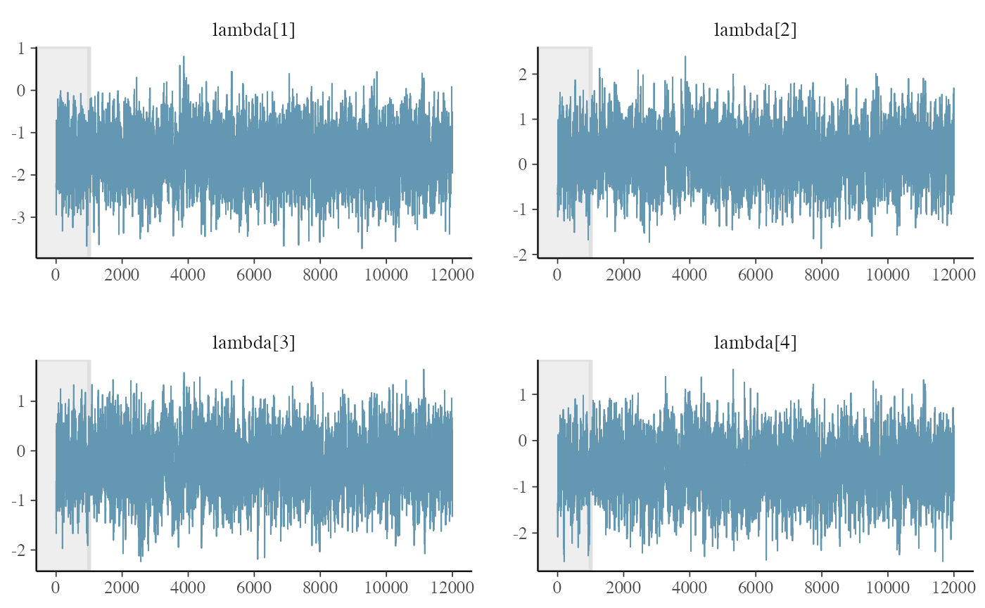

They sound ok so there is no reason why we should not trust our data

Ranking with the bt model

Let’s get the rank with the simple bt model

get_rank_of_players_table(m1, format = 'html')

Estimated posterior ranks
Parameter	MedianRank	MeanRank	StdRank
Flamengo	1	1.596	1.003
Palmeiras	3	3.286	1.934
Santos	3	3.139	1.870
São Paulo	4	4.850	2.460
Athlético-PR	6	6.601	2.808
Corinthians	7	7.346	3.036
Grêmio	7	7.379	3.134
Internacional	8	8.333	3.224
Fluminense	9	9.458	3.207
Fortaleza	9	9.539	3.311
Vasco	11	10.476	3.202
Goiás	12	11.676	3.175
Cruzeiro	13	12.675	3.038
Atlético-MG	14	13.699	2.930
Bahia	14	13.711	2.943
Botafogo-rj	16	15.556	2.539
Ceará	16	15.516	2.584
Chapecoense	18	17.804	1.748
CSA	18	17.747	1.814
Avaí	20	19.613	0.823

Fitting the Davidson model

Now lets investigate how ties impact our model

m2 <- bpc(d, 
          player0 = 'VisitorTeam', 
          player1 =  'HomeTeam', 
          player0_score = 'ScoreVisitorTeam',
          player1_score = 'ScoreHomeTeam',
          model_type = 'davidson',
          solve_ties = 'none',
          priors = list(prior_lambda_std=2.0), # making a more informative prior to improve convergence
          iter = 3000) #stan indicates a low bulk ESS so we are increasing the number of iterations
#> Running MCMC with 4 parallel chains...
#> 
#> Chain 2 finished in 28.4 seconds.
#> Chain 3 finished in 28.5 seconds.
#> Chain 1 finished in 29.2 seconds.
#> Chain 4 finished in 29.4 seconds.
#> 
#> All 4 chains finished successfully.
#> Mean chain execution time: 28.8 seconds.
#> Total execution time: 29.6 seconds.

For sake of space and repetition we will not present the diagnostics which can be observed at:

launch_shinystan(m2)

Let’s look at the parameters

print(m2)
#> Estimated baseline parameters with 95% HPD intervals:
#> 
#> Table: Parameters estimates
#> 
#> Parameter                  Mean   Median   HPD_lower   HPD_higher
#> ----------------------  -------  -------  ----------  -----------
#> lambda[Avaí]             -1.924   -1.918      -3.241       -0.567
#> lambda[Internacional]     0.157    0.166      -1.077        1.378
#> lambda[Cruzeiro]         -0.697   -0.684      -2.020        0.489
#> lambda[Botafogo-rj]      -0.595   -0.587      -1.865        0.670
#> lambda[Vasco]            -0.072   -0.073      -1.230        1.232
#> lambda[Corinthians]       0.291    0.292      -0.964        1.463
#> lambda[CSA]              -1.112   -1.100      -2.451        0.109
#> lambda[Goiás]            -0.074   -0.072      -1.247        1.232
#> lambda[Fortaleza]         0.125    0.130      -1.143        1.335
#> lambda[Santos]            1.069    1.071      -0.207        2.350
#> lambda[Grêmio]            0.623    0.617      -0.638        1.866
#> lambda[Palmeiras]         1.232    1.228      -0.013        2.545
#> lambda[Atlético-MG]      -0.059   -0.050      -1.288        1.211
#> lambda[Chapecoense]      -0.994   -0.992      -2.312        0.241
#> lambda[Ceará]            -0.733   -0.719      -1.963        0.527
#> lambda[Athlético-PR]      0.711    0.716      -0.558        1.922
#> lambda[Flamengo]          2.031    2.025       0.695        3.431
#> lambda[São Paulo]         0.606    0.612      -0.716        1.801
#> lambda[Bahia]            -0.146   -0.138      -1.433        1.038
#> lambda[Fluminense]       -0.389   -0.376      -1.703        0.812
#> nu                        0.388    0.390       0.151        0.616
#> NOTES:
#> * A higher lambda indicates a higher team ability
#> * Large positive values of the nu parameter indicates a high probability of tie regardless of the abilities of theplayers.
#> * Large negative values of the nu parameter indicates a low probability of tie regardless of the abilities of the players.
#> * Values of nu close to zero indicate that the probability of tie is more dependable on abilities of the players. If nu=0 the model reduces to the Bradley-Terry model.

Ranking

Let’s look at the ranking with ties:

get_rank_of_players_table(m2, format = 'html')

Estimated posterior ranks
Parameter	MedianRank	MeanRank	StdRank
Flamengo	1	1.341	0.751
Palmeiras	3	3.151	1.800
Santos	3	3.788	2.214
Athlético-PR	5	5.499	2.660
Grêmio	5	5.962	2.905
São Paulo	6	6.131	2.852
Corinthians	8	8.328	3.191
Fortaleza	9	9.331	3.370
Internacional	9	9.359	3.413
Atlético-MG	11	10.939	3.488
Goiás	11	10.805	3.445
Vasco	11	10.954	3.453
Bahia	12	11.434	3.524
Fluminense	14	13.157	3.393
Botafogo-rj	15	14.749	2.822
Ceará	16	15.477	2.777
Cruzeiro	16	15.410	2.785
Chapecoense	18	17.059	2.302
CSA	18	17.456	2.130
Avaí	20	19.670	0.767

We can see that when we consider ties the rank has changed a bit and the difference between the teams reduce (we can see from both the parameter table as well as many equal median ranks between the teams).

Bradley-Terry with order effect (home advantage)

d_home <- d %>% 
  dplyr::mutate(home_player1 = 1)

m3 <- bpc(d_home, 
          player0 = 'VisitorTeam', 
          player1 =  'HomeTeam', 
          player0_score = 'ScoreVisitorTeam',
          player1_score = 'ScoreHomeTeam',
          z_player1 = 'home_player1',
          model_type = 'bt-ordereffect',
          solve_ties = 'random',
          priors = list(prior_lambda_std=2.0), # making a more informative prior to improve convergence
          iter = 3000) #stan indicates a low bulk ESS so we are increasing the number of iterations
#> Running MCMC with 4 parallel chains...
#> 
#> Chain 3 finished in 33.9 seconds.
#> Chain 4 finished in 33.9 seconds.
#> Chain 1 finished in 34.2 seconds.
#> Chain 2 finished in 34.3 seconds.
#> 
#> All 4 chains finished successfully.
#> Mean chain execution time: 34.1 seconds.
#> Total execution time: 34.4 seconds.

For sake of space and repetition we will not present the diagnostics which can be observed at:

launch_shinystan(m3)

Let’s look at the parameters

print(m3)
#> Estimated baseline parameters with 95% HPD intervals:
#> 
#> Table: Parameters estimates
#> 
#> Parameter                  Mean   Median   HPD_lower   HPD_higher
#> ----------------------  -------  -------  ----------  -----------
#> lambda[Avaí]             -1.291   -1.287      -2.414       -0.125
#> lambda[Internacional]     0.312    0.318      -0.818        1.353
#> lambda[Cruzeiro]         -0.153   -0.153      -1.254        0.920
#> lambda[Botafogo-rj]      -0.625   -0.623      -1.737        0.446
#> lambda[Vasco]            -0.150   -0.153      -1.284        0.887
#> lambda[Corinthians]       0.432    0.430      -0.691        1.522
#> lambda[CSA]              -0.873   -0.862      -1.984        0.236
#> lambda[Goiás]            -0.153   -0.153      -1.267        0.935
#> lambda[Fortaleza]         0.078    0.077      -1.021        1.150
#> lambda[Santos]            0.810    0.808      -0.299        1.940
#> lambda[Grêmio]            0.312    0.311      -0.803        1.382
#> lambda[Palmeiras]         0.555    0.553      -0.532        1.651
#> lambda[Atlético-MG]      -0.150   -0.143      -1.241        0.940
#> lambda[Chapecoense]      -0.750   -0.746      -1.848        0.356
#> lambda[Ceará]            -0.504   -0.508      -1.575        0.619
#> lambda[Athlético-PR]     -0.036   -0.035      -1.126        1.049
#> lambda[Flamengo]          1.724    1.718       0.549        2.952
#> lambda[São Paulo]         0.432    0.437      -0.705        1.482
#> lambda[Bahia]            -0.274   -0.263      -1.332        0.822
#> lambda[Fluminense]       -0.270   -0.267      -1.373        0.806
#> gm                       -0.491   -0.491      -0.723       -0.268
#> NOTES:
#> * A higher lambda indicates a higher team ability
#> * Large positive values of the gm parameter indicate that player 1 has a disadvantage. E.g. in a home effect scenario positive values indicate a home disadvantage.
#> * Large negative values of the gm parameter indicate that player 1 has an advantage. E.g. in a home effect scenario negative values indicate a home advantage.
#> * Values of gm close to zero indicate that the order effect does not influence the contest. E.g. in a home effect it indicates that player 1 does not have a home advantage nor disadvantage.

We can see that the gm parameter is negative indicating that playing home indeed provide an advantage to the matches.

Ranking

Let’s look at the ranking with home advantage:

get_rank_of_players_table(m3, format = 'html')

Estimated posterior ranks
Parameter	MedianRank	MeanRank	StdRank
Flamengo	1.0	1.080	0.340
Santos	3.0	3.217	1.862
Palmeiras	4.0	4.885	2.652
Corinthians	5.0	5.917	3.010
São Paulo	5.0	5.767	3.066
Grêmio	6.0	6.808	3.264
Internacional	6.0	6.780	3.159
Fortaleza	9.0	8.883	3.497
Athlético-PR	10.0	10.223	3.688
Cruzeiro	11.5	11.472	3.783
Atlético-MG	12.0	11.603	3.588
Goiás	12.0	11.555	3.691
Vasco	12.0	11.552	3.547
Bahia	13.0	12.739	3.568
Fluminense	13.0	12.673	3.397
Ceará	15.0	14.803	3.162
Botafogo-rj	17.0	16.112	2.791
Chapecoense	18.0	16.854	2.518
CSA	18.0	17.702	2.148
Avaí	20.0	19.375	1.115

We can see that the players ranking has changed a bit from the BT and the Davidson model when we compensate for the home advantage

Davidson with order effect (home advantage)

Now let’s fit our last model. The Davidson model with order effect. Here we take into account the ties and the home advantage effect

m4 <- bpc(d_home, 
          player0 = 'VisitorTeam', 
          player1 =  'HomeTeam', 
          player0_score = 'ScoreVisitorTeam',
          player1_score = 'ScoreHomeTeam',
          z_player1 = 'home_player1',
          model_type = 'davidson-ordereffect',
          solve_ties = 'none',
          priors = list(prior_lambda_std=2.0), # making a more informative prior to improve convergence
          iter = 3000) #stan indicates a low bulk ESS so we are increasing the number of iterations
#> Running MCMC with 4 parallel chains...
#> 
#> Chain 1 finished in 33.7 seconds.
#> Chain 4 finished in 33.7 seconds.
#> Chain 2 finished in 34.0 seconds.
#> Chain 3 finished in 34.4 seconds.
#> 
#> All 4 chains finished successfully.
#> Mean chain execution time: 34.0 seconds.
#> Total execution time: 34.6 seconds.

For sake of space and repetition we will not present the diagnostics which can be observed at:

launch_shinystan(m4)

Let’s look at the parameters

print(m4)
#> Estimated baseline parameters with 95% HPD intervals:
#> 
#> Table: Parameters estimates
#> 
#> Parameter                  Mean   Median   HPD_lower   HPD_higher
#> ----------------------  -------  -------  ----------  -----------
#> lambda[Avaí]             -3.014   -2.998      -4.621       -1.381
#> lambda[Internacional]     0.012    0.004      -1.426        1.459
#> lambda[Cruzeiro]         -1.008   -1.000      -2.501        0.489
#> lambda[Botafogo-rj]      -0.806   -0.795      -2.314        0.642
#> lambda[Vasco]            -0.034   -0.040      -1.513        1.396
#> lambda[Corinthians]       0.377    0.365      -1.052        1.844
#> lambda[CSA]              -1.617   -1.606      -3.161       -0.103
#> lambda[Goiás]            -0.026   -0.027      -1.469        1.431
#> lambda[Fortaleza]         0.371    0.374      -1.095        1.843
#> lambda[Santos]            1.408    1.406      -0.035        2.954
#> lambda[Grêmio]            0.957    0.953      -0.614        2.388
#> lambda[Palmeiras]         1.822    1.815       0.238        3.302
#> lambda[Atlético-MG]       0.162    0.160      -1.373        1.575
#> lambda[Chapecoense]      -1.235   -1.227      -2.701        0.311
#> lambda[Ceará]            -1.183   -1.185      -2.763        0.282
#> lambda[Athlético-PR]      1.155    1.156      -0.358        2.642
#> lambda[Flamengo]          2.813    2.791       1.221        4.545
#> lambda[São Paulo]         0.775    0.778      -0.781        2.219
#> lambda[Bahia]            -0.376   -0.381      -1.811        1.097
#> lambda[Fluminense]       -0.768   -0.761      -2.191        0.778
#> gm                       -3.900   -3.873      -4.883       -2.959
#> nu                        0.086    0.085      -0.125        0.298
#> NOTES:
#> * A higher lambda indicates a higher team ability
#> * Large positive values of the nu parameter indicates a high probability of tie regardless of the abilities of theplayers.
#> * Large negative values of the nu parameter indicates a low probability of tie regardless of the abilities of the players.
#> * Values of nu close to zero indicate that the probability of tie is more dependable on abilities of the players. If nu=0 the model reduces to the Bradley-Terry model.
#> * Large positive values of the gm parameter indicate that player 1 has a disadvantage. E.g. in a home effect scenario positive values indicate a home disadvantage.
#> * Large negative values of the gm parameter indicate that player 1 has an advantage. E.g. in a home effect scenario negative values indicate a home advantage.
#> * Values of gm close to zero indicate that the order effect does not influence the contest. E.g. in a home effect it indicates that player 1 does not have a home advantage nor disadvantage.

We can see again that the home advantage gm parameter was negative, indicating that there is a home advantage effect.

Ranking

Let’s look at the ranking with home advantage and ties:

get_rank_of_players_table(m4, format = 'html')

Estimated posterior ranks
Parameter	MedianRank	MeanRank	StdRank
Flamengo	1	1.301	0.718
Palmeiras	2	2.819	1.506
Santos	4	4.069	2.086
Athlético-PR	5	5.150	2.510
Grêmio	5	5.684	2.627
São Paulo	6	6.502	2.831
Corinthians	8	8.470	3.231
Fortaleza	8	8.516	3.157
Atlético-MG	9	9.459	3.283
Goiás	10	10.454	3.268
Internacional	10	10.435	3.120
Vasco	11	10.505	3.180
Bahia	13	12.453	3.159
Botafogo-rj	15	14.449	3.029
Fluminense	15	14.237	2.909
Cruzeiro	16	15.509	2.621
Ceará	17	16.226	2.458
Chapecoense	17	16.422	2.411
CSA	18	17.521	2.014
Avaí	20	19.819	0.555

Comparing the models with WAIC

Let’s see now using an information criteria (the WAIC) which model fits the data better.

m1_waic <-get_waic(m1)
m2_waic <-get_waic(m2)
m3_waic <-get_waic(m3)
m4_waic <-get_waic(m4)

We can look at each waic:

m1_waic
#> 
#> Computed from 12000 by 380 log-likelihood matrix
#> 
#>           Estimate   SE
#> elpd_waic   -246.6  8.3
#> p_waic        19.6  0.9
#> waic         493.1 16.6
m2_waic
#> 
#> Computed from 12000 by 380 log-likelihood matrix
#> 
#>           Estimate   SE
#> elpd_waic   -332.5 10.4
#> p_waic        19.7  1.1
#> waic         664.9 20.7
m3_waic
#> 
#> Computed from 12000 by 380 log-likelihood matrix
#> 
#>           Estimate   SE
#> elpd_waic   -246.5  8.2
#> p_waic        20.8  0.9
#> waic         492.9 16.5
m4_waic
#> 
#> Computed from 12000 by 380 log-likelihood matrix
#> 
#>           Estimate   SE
#> elpd_waic   -242.1  7.5
#> p_waic        17.0  0.7
#> waic         484.3 15.0

Or can also use the loo::compare function to see which performs better.

loo::loo_compare(m1_waic,m2_waic, m3_waic, m4_waic)
#>        elpd_diff se_diff
#> model4   0.0       0.0  
#> model3  -4.3       7.2  
#> model1  -4.4       6.3  
#> model2 -90.3       7.4

Home advantage in the Bradley-Terry and in the Davidson model

Introduction

Fitting a Bradley-Terry model

Simple diagnostics

Ranking with the bt model

Fitting the Davidson model

Ranking

Bradley-Terry with order effect (home advantage)

Ranking

Davidson with order effect (home advantage)

Ranking

Comparing the models with WAIC